El Condor Y el Gamma

El Condor y el Gamma (*)

Mathematica Mathematica

The function under consideration is coded with Mathematica:

condor[x_, y_] := 
  Module[{a, b, c, d, e, alpha, beta},

  e = Gamma[y + 1];
  a = Gamma[1/2*y - 1/2*x + 1/2];
  b = Gamma[-1/2*x + 1/2*y + 1];
  c = Gamma[1/2*x + 1/2*y + 1/2];
  d = Gamma[1/2*x + 1/2*y + 1];
  
  alpha = Cos[Pi*(y - x)];
  beta  = Cos[Pi*(y + x)];
  
  Log[e] + Log[a]*((alpha - 1)/2) 
+ Log[b]*((-alpha - 1)/2) 
+ Log[c]*((beta-1)/2)+Log[d]*((-beta-1)/2) 
  ]

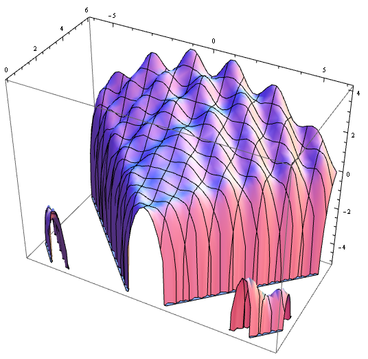
On the right hand side you see two different 3D plots.
The first one is

Plot3D[condor[x, y], {x, -6, 6}, {y, 0, 6},
BoxRatios -> Automatic
]

However, this is not the intended plot. We want to plot the
function condor[x,y] only for x = -y .. y, where y = 0 .. 6.
This can be achieved by the option 'RegionFunction'.


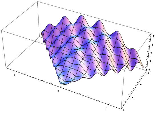
Plot3D[condor[x, y], {x, -6, 6}, {y, 0, 6}, 
BoxRatios -> Automatic,
RegionFunction -> Function[{x,y,z},-y<=x<=y]
]

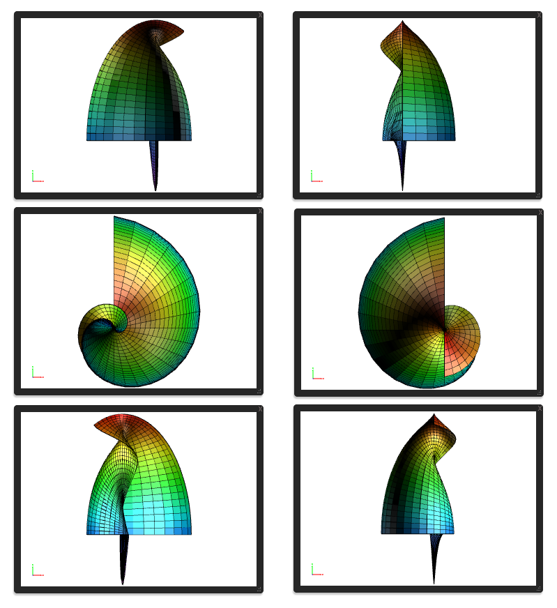
The definition of some views

View	Axes	Azimuth	Zenith	View Direction
Top		-90°	0°	(0 \| 0 \| 1)
Bottom		90°	180°	(0 \| 0 \| -1)
Front		-90°	90°	(0 \| -1 \| 0)
Back		90°	90°	(0 \| 1 \| 0)
Right		0°	90°	(1 \| 0 \| 0)
Left		180°	90°	(-1 \| 0 \| 0)

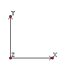
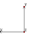
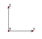
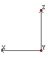
`Orientation´ as used by Maple specifies
the theta and phi angles of the point in
3-dimensions from which the plot is to
be viewed.

The default is at a point that is out
perpendicular from the screen
(negative z axis) so that the entire surface
can be seen. The point is described in
spherical coordinates where theta and
phi are angles in degrees. (θ, φ)

Below we compare Asymptote 3D plots
(on the left hand side) with Maple 3D
plots (on the right hand side).

The plots were made with Asymptote
version 1.72 using movie15.sty version
2009-05-15 and with Maple V R5 (1998)
respectively.

The plot at the top of the right hand side
was post processed (light and anti-aliasing)
with JavaView. The engine behind the
display of the applet is also JavaView.

Asymptote Maple

 
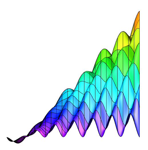
// Compiled with Asymptote version 1.86.

import palette;
import graph3;

triple Condor(pair t) {
   real y = t.y, x = t.x*y;
   real e = gamma(y+1), ymx = y - x, ypx = y + x;
   real a = gamma((ymx+1)/2), b = gamma((ymx+2)/2);
   real c = gamma((ypx+1)/2), d = gamma((ypx+2)/2);
   real A = cos(pi*ymx), B = cos(pi*ypx);
   real z = log(e)+log(a)*((A-1)/2)+log(b)*((-A-1)/2)
            +log(c)*((B-1)/2)+log(d)*((-B-1)/2);
   return (x, y, z);
}

void Plot3DAsy(projection proj, string name) {
   size(300, 300, IgnoreAspect);
   currentprojection = proj;
   surface s = surface(Condor,(-1,0),(1,7),16,Spline);
   s.colors(palette(s.map(zpart), Rainbow()));
   draw(s);
   // axes3("$x$","$y$","$z$",red); 
   shipout("Condor" + name);
}

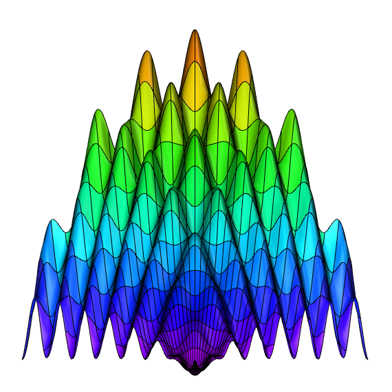
Plot3DAsy(FrontView,"Front");

// Plot3DAsy(LeftView,"Left");
// Plot3DAsy(RightView,"Right");
// Plot3DAsy(BackView,"Back");
// Plot3DAsy(BottomView,"Bottom");
// Plot3DAsy(TopView,"Top");

//
// projection SpecialView() {
// triple camera = (38.51, 11.61, -5.20); 
// triple up     = (-0.0135, -0.005, -0.0197); 
// triple target = (0.0, 0.0, 0.0); 
// return perspective(camera, up,target,autoadjust=false);
// }  Plot3DAsy(SpecialView(),"Special");

 

 condor := proc(x,y) 
 local a, b, c, d, e, alpha, beta;

 e := GAMMA(y+1);
 a := GAMMA(1/2*y-1/2*x+1/2); 
 b := GAMMA(-1/2*x+1/2*y+1);
 c := GAMMA(1/2*x+1/2*y+1/2); 
 d := GAMMA(1/2*x+1/2*y+1);

 alpha := cos(Pi*(y-x)); 
 beta  := cos(Pi*(y+x));

 log(e)+log(a)*((alpha-1)/2)+log(b)*
 ((-alpha-1)/2)+log(c)*((beta-1)/2)+
 log(d)*((-beta-1)/2) end;
 
__________________________________________

 
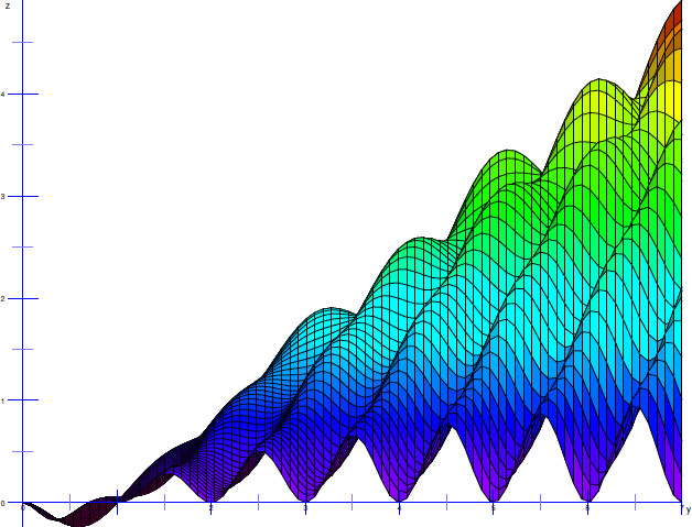
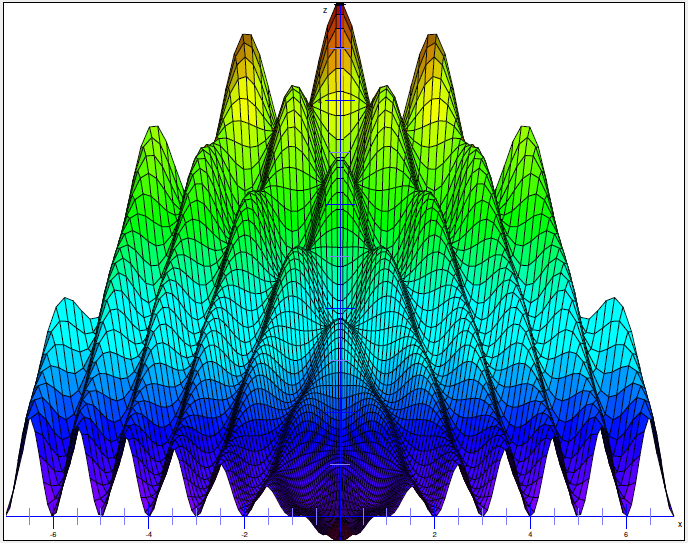
 plot3dMaple := proc(view) local theta, phi;
 
   if(view = "top")    then theta := -90; phi := 0   # +x+y
 elif(view = "bottom") then theta :=  90; phi := 180 # -x+y
 
 elif(view = "front") then theta := -90; phi := 90 # +x+z
 elif(view = "back")  then theta :=  90; phi := 90 # -x+z
 
 elif(view = "right") then theta :=   0; phi := 90 # +y+z
 elif(view = "left")  then theta := 180; phi := 90 # -y+z
 
 elif(view = "special") then theta := -145; phi := -105 fi; 

 plot3d(condor(x, y), x = -y..y, y = 0..8, 
        orientation = [theta, phi],
        axes = BOXED, grid = [64,64] ); 
 end;

Asymptote Maple

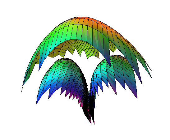
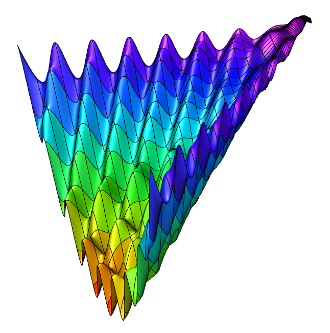
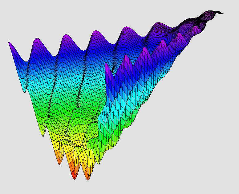
Plot3DAsy("Special"); plot3dMaple("special");

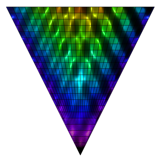
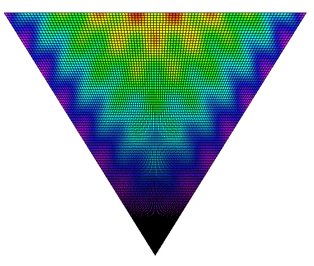
Plot3DAsy("Top"); plot3dMaple("top");

Plot3DAsy("Right"); plot3dMaple("right");

Plot3DAsy("Front"); plot3dMaple("front");

settings.toolbar=false; 
import palette; 
import graph3; 
 
picture pic; 
currentlight = adobe; 
size(pic, 800, 400); 
 
void addAllStdViews(picture dest, picture src, 
     bool group=true, filltype filltype=NoFill, 
     bool above=true)  
{  
    frame addFrame(frame F, real x, real y=0) { 
    add(dest,shift(x,y)*F,group,filltype,above); 
    return F;}  
 
	real h, r, u, s = 50; 
 
	frame F = addFrame(src.fit(FrontView), 0);  
	h = max(F).y - min(F).y; 
	r = max(F).x - min(F).x + 2*s; 
 
	F = addFrame(src.fit(TopView), r); 
	h = max(h, max(F).y - min(F).y); 
	u = r + max(F).x - min(F).x + s; 
 
	F = addFrame(src.fit(RightView), u); 
	h = -max(h, max(F).y - min(F).y); 
 
	F = addFrame(src.fit(BackView), 0, h);  
	F = addFrame(src.fit(BottomView), r, h); 
	F = addFrame(src.fit(LeftView), u, h);  
}  

triple dervish(pair t) 
{ 
	real x = t.x*sin(t.x)*cos(t.y); 
	real y = t.x*cos(t.x)*cos(t.y); 
	real z = log(t.x^6+0.01)*sin(t.y); 
	return (x, y, z); 
} 

   pair H =(0,0), L =(2*pi, 2);   
   surface s = surface(dervish, L, H, 32); 
   s.colors(palette(s.map(zpart), Rainbow())); 
   draw(pic, s, meshpen = black); 
   addAllStdViews(currentpicture, pic);

Multiple views in one picture. Multiple views of the "dervish".

Condor.pdf

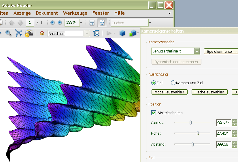
Applet shows Condor.jvx

You will need Adobe Reader 9 or later to view this pdf file! Move mouse into the applet, right click 'New Display' for more options. Enlarge! Close via menu: File & Close, not via the window's X. Otherwise the browser might harmlessly freeze for some seconds.

Ovid, me and my pet condor like the metamorphosis.
Here are some of the transformations the condor went through:

typedef triple Transform3D(triple t);

triple Spherical(triple t)
{
   real x = t.x*cos(t.y)*sin(t.z);
   real y = t.x*sin(t.y)*sin(t.z);
   real z = t.x*cos(t.z);
   return (x, y, z);
}

triple MaxwellCylindrical(triple t)
{
   real x = 1/pi*(t.x+1+exp(t.x)*cos(t.y));
   real y = 1/pi*(t.y+exp(t.x)*sin(t.y));
   real z = t.z;
   return (x, y, z);
}

triple InvCassiniCylindrical(triple t)
{
   real a = 1;
   real x = a*2^(1/2)/2*((exp(2*t.x)
            +2*exp(t.x)*cos(t.y)+1)^(1/2) +
            exp(t.x)*cos(t.y)+1)^(1/2)/(exp(2*t.x)
            +2*exp(t.x)*cos(t.y)+1)^(1/2);
   real y = a*2^(1/2)/2*((exp(2*t.x)+2*exp(t.x)*
            cos(t.y)+1)^(1/2) - exp(t.x)*cos(t.y)-1)^(1/2)
            /(exp(2*t.x)+2*exp(t.x)*cos(t.y)+1)^(1/2);
   return (x, y, t.z);
}

triple BipolarCylindrical(triple t)
{
   real h = cosh(t.y) - cos(t.x);
   if( h == 0) h = 1;
   real x = sinh(t.y) / h;
   real y = sin(t.x) / h;
   return (x, y, t.z);
}

triple Ellipsoidal(triple t)
{
   real a = 1, b = 1/2;
   real x = t.x*t.y*t.z/(a*b);
   real y = abs((t.x^2-b^2)*(t.y^2-b^2)*(b^2-t.z^2)
            /(a^2-b^2))^(1/2)/b;
   real z = abs((t.x^2-a^2)*(a^2-t.y^2)*(a^2-t.z^2)
            /(a^2-b^2))^(1/2)/a;
   return (x, y, z);
}

To plot the transformed condor I call, respectively:

Plot3D(Condor,InvCassiniCylindrical,
       "Front","CondorInvCass");
Plot3D(Condor,BipolarCylindrical,
       "Right","CondorBipolCyl");
Plot3D(Condor,Ellipsoidal,
       "Front","CondorEllip" );
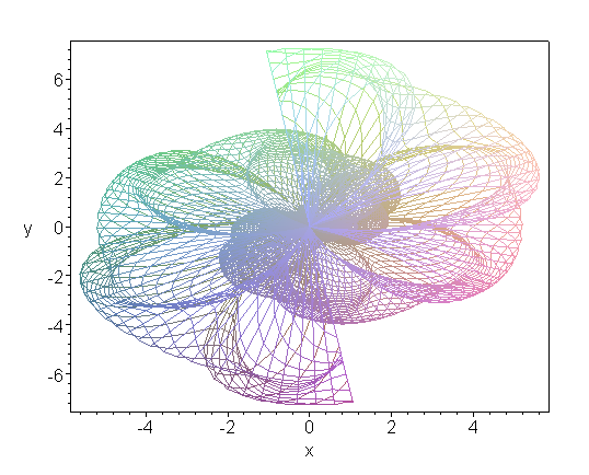
Plot3D(Condor,Spherical,
       "Front","CondorSph" );
PlotAllViews(Condor,"Condor");

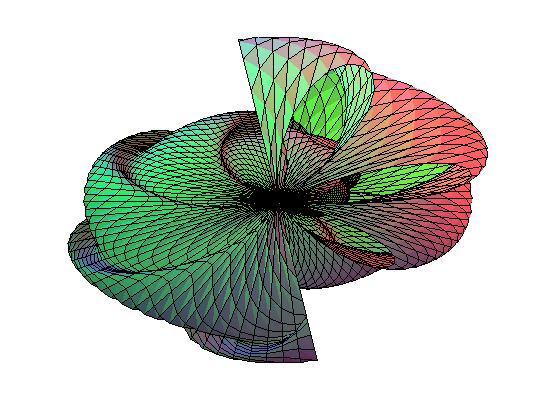
void Plot3D(Function3D f, Transform3D t, string proj, string funname) { write("Plotting: " + funname + proj); size(Size, Size, IgnoreAspect); currentprojection = SetView(proj); triple tf(pair p) { return t(f(p)); } surface s = surface(tf, L, H, Grid); s.colors(palette(s.map(zpart), Rainbow())); draw(s, meshpen = black); shipout(funname + proj); erase(); }

In column at the right hand side the SphericalCondor is plotted. Amazing, isn't it? At least when you know my condor :-) And some of the other transformations lead to other equal astonishing results. The full asy-worksheet can be downloaded here.

The SphericalCondor (plotted with Maple):

Below is the amazing condor in it's ellipsoidal form as plotted by Maple.

The function name `condor´ is a (TM) of Peter Luschny ;-). As far as I know this is a new function. The function has a remarkable mathematical background. If you use it please give reference to the author. The function is discussed in my forthcoming paper "Swing, divide and conquer the factorial".
(*) El Condor y el Gamma was the code name for the generalization of the binomial coefficients proposed by the author in the cited paper. And yes, the triangle displayed above is Pascal's triangle when discretized. So in fact you literally looked behind this amazing triangle in the plots above. So look again at the plot.

The Condor as drawn by Leonardo. The Night Condor.