Generalized Bernoulli
Numbers and Polynomials
This is the third part of a series of posts which build on each other.
It is recommended that the reader skims through the previous parts first to become familiar with the definitions and notations given there which we will not repeat here.
The generalized Bernoulli numbers
The Bernoulli numbers (Concrete Mathematics, section 6.5), which are rational numbers, can be generalized via the Stirling-Frobenius subset numbers.
$$\operatorname{B}^{(m)}_n = \sum_{k=0}^n \frac{(-m)^k }{k+1} k! \genfrac\{\}{0pt}{}{n}{k}_m = \sum_{k=0}^n \frac{(-1)^k}{k+1} \sum_{j=0}^{n} \genfrac < > {0pt}{}{n}{j}_m \genfrac ( ) {0pt}{}{j}{n-k}. $$
We will call these numbers the generalized Bernoulli numbers. In the case $m=1$ we will suppress the index $m$ and write
$$\operatorname{B}_n = \sum_{k=0}^n \frac{(-1)^k }{k+1} k! \genfrac\{\}{0pt}{}{n}{k} = \sum_{k=0}^n \frac{(-1)^k}{k+1} \sum_{j=0}^{n} \genfrac < > {0pt}{}{n}{j} \genfrac ( ) {0pt}{}{j}{n-k}. $$
These are the classical Bernoulli numbers by a theorem due to Frobenius relating Eulerian numbers $\genfrac < > {0pt}{}{n}{k}$ to Stirling set numbers $\genfrac\{\}{0pt}{}{n}{k}$. We use notations introduced by D. Knuth.
|
|
To simplify things we will use the Clausen numbers $ \operatorname{C}_n$ as the common denominators for all $ \operatorname{B}^{(m)}_n$. The Clausen numbers are defined as $ \operatorname{C}_0 =1 $ and for $n \ge 1$ as $\operatorname{C}_n = \prod_{ p - 1 | n} p $ where p is prime (A027760, see also A160014).
$$ \operatorname{C}_n = 1,\, 2,\, 6,\, 2,\, 30,\, 2,\, 42,\, 2,\, 30,\, 2,\, 66,\, 2,\, 2730,\, 2,\, 6,\, 2,\, 510,\, 2,\, 798,\, 2,... $$This means, for instance, that we will not reduce $\operatorname{B}^{(2)}_{n}$ to lowest terms but will write the numbers in the form (see A225480 for the numerators):
$$ \operatorname{B}^{(2)}_n = 1, 0, \frac{-2}{6}, 0, \frac{14}{30}, 0, \frac{-62}{42}, 0, \frac{254}{30}, 0, \frac{-5110}{66}, 0, \frac{2828954}{2730} ...$$Of course it requires a proof that this is possible. For $m=1$ this is the famous von Staudt-Clausen theorem and for $m >1$ this follows from the fact that the denominator of $\operatorname{B}^{(m)}_{n}$ divides $ \operatorname{C}_n$. In other words we have a generalization of the von Staudt-Clausen theorem from "For $n\ge 0:\, \operatorname{denom} \operatorname{B}_n^{(1)}=\operatorname{C}_n $" to "For $ m \ge1$ and $n \ge 0:\,$ $ \operatorname{denom} \operatorname{B}_n^{(m)}$ divides $ \operatorname{C}_n.$ "
| Clausen-normalized numerators of $\operatorname{B}^{(m)}_n$ |
0 | 1 | 2 | 3 | 4 | 5 | 6 | 7 |
| $ m=1 $, A027641 | 1 | -1 | 1 | 0 | -1 | 0 | 1 | 0 |
| $ m=2 $, A225480 | 1 | 0 | -2 | 0 | 14 | 0 | -62 | 0 |
| $ m=3 $ | 1 | 1 | -3 | -2 | 39 | 10 | -363 | -98 |
| $ m=4 $ | 1 | 2 | -2 | -6 | 14 | 50 | -62 | -854 |
| $ m=5 $ | 1 | 3 | 1 | -12 | -145 | 148 | 4537 | -3892 |
| $ m=6 $ | 1 | 4 | 6 | -20 | -546 | 340 | 22506 | -12740 |
| $ m=7 $ | 1 | 5 | 13 | -30 | -1321 | 670 | 71533 | -33910 |
The table above can be computed with Sage and this script:
def Clausen(n):   # -- The Clausen numbers --
    if n == 0: return 1
    return mul(filter(lambda s: is_prime(s), map(lambda i: i+1, divisors(n))))

def ClausenB(n):  # -- Clausen numbers, implementation better to read but much slower --
    return mul(filter(lambda p: n%(p-1) == 0, primes(n+2)))

@CachedFunction
def EulerianNumber(n, k, m) :   # -- The generalized Eulerian numbers --
    if n == 0: return 1 if k == 0 else 0
    return (m*(n-k)+m-1)*EulerianNumber(n-1,k-1,m) + (m*k+1)*EulerianNumber(n-1,k,m)

def gen_bernoulli_number(n, m):   # -- The generalized Bernoulli numbers --
    return add(add(EulerianNumber(n, j, m)*binomial(j, n - k)
           for j in (0..n))*(-1)^k/(k+1) for k in (0..n))

for m in (1..7): [gen_bernoulli_number(n,m)*Clausen(n) for n in (0..7)]
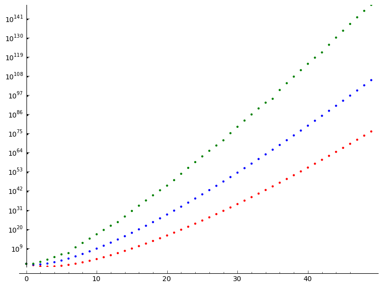
Plotting abs(gen_bernoulli_number(2n, m)) for $0 \le n \le 50$ and $1 \le m \le 3$ with the vertical axis in logarithmic scale we see how fast the numbers grow in size (the graph of the classical Bernoulli numbers is red):

Note that $ \operatorname{B}^{(2)}_{2n} = \operatorname{B}^{(4)}_{2n}$ for $n \ge 0 $. Moreover the $ \operatorname{B}^{(4)}_{2n+1} $ are integers. Thus $ \operatorname{B}^{(4)}_{n} - \operatorname{B}^{(2)}_{n}$ is the integer sequence
$$ 0, \, 1, \, 0, \, -3,\, 0,\, 25,\, 0,\, -427,\, 0,\, 12465,\, 0,\, -555731,\, 0,\, ... $$This is up to sign A009843 (Egf. x/cos(x)), but more exciting these are the numerators of the lost Bernoulli numbers as I called them in my blog post on the Euler-Bernoulli diamond, the numerators of the Bernoulli secant numbers A009843 / A193476.
The observation that $ \operatorname{B}^{(4)}_{2n+1}$ are integers is just a special case of a much more general fact: All $\, \operatorname{B}^{(m)}_{2n+1} $ are integers for $m \ge 1$ and $n \ge 1$. Thus the Bernoulli numbers are only semi-rationals (pardon the expression), a fact which is of no great importance in the classical case because all classical Bernoulli numbers with an odd index $n \gt 1$ are zero.
| m \ n | 1 | 2 | 3 | 4 | 5 | 6 | 7 |
| 3 | -1 | 5 | -49 | 809 | -20317 | 722813 | -34607305 |
| 4 | -3 | 25 | -427 | 12465 | -555731 | 35135945 | -2990414715 |
| 5 | -6 | 74 | -1946 | 88434 | -6154786 | 607884394 | -80834386026 |
| 6 | -10 | 170 | -6370 | 415826 | -41649850 | 5922729722 | -1134081384850 |
| 7 | -15 | 335 | -16955 | 1503963 | -204957775 | 39666688711 | -10337889346275 |
Fortunately all these sequences can be computed by a single formula:
$$ \operatorname{B}^{(m)}_{2n+1} = - \sum_{k=0}^{2n+1} \binom{2n+1}{k} \operatorname{B}_{k} m^k $$
These sequences can be found (modulo sign, offset, suppressed zeros and other OEIS-typical peculiarities) in A002111, A009843, A069852, A069994, A083011, A083012, A083013, A083014. But much more is true.
$$ \operatorname{B}^{(m)}_{n} = (-1)^n \sum_{k=0}^{n} \binom{n}{k} \operatorname{B}_{k} m^k \quad ( n \gt 0, \ m \gt 0) $$
With regard to the Stirling-Frobenius numbers and generalized Eulerian numbers we thus have the identities
| $$ \sum_{k=0}^n \frac{(-m)^{k} }{k+1} k! \genfrac\{\}{0pt}{}{n}{k}_m = \sum_{k=0}^n \frac{(-1)^{k}}{k+1} \sum_{j=0}^{n} \genfrac < > {0pt}{}{n}{j}_m \genfrac ( ) {0pt}{}{j}{n-k} = (-1)^n \sum_{k=0}^{n} \binom{n}{k} \operatorname{B}_{k} m^k. $$ | (I) |
This proves that our choice of the parameter m in generalizing the Eulerian numbers and the Stirling numbers was a sensible choice.
But wait a minute! Aren't the polynomials $\sum_{k=0}^{n} \binom{n}{k} \operatorname{B}_{k} x^k$ the Bernoulli polynomials? Despite the appearance they are not. Anyway, let us experiment a little bit: What happens if we replace the Bernoulli numbers in the formula by the Bernoulli polynomials?
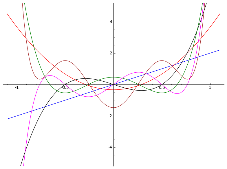
Generalized Bernoulli polynomials $ \operatorname{B}_{n,2}(x).$
More precisely we define the generalized Bernoulli polynomials as
| $$ \operatorname{B}_{n,m}(x) = \sum_{k=0}^n \sum_{j=0}^k \sum_{v=0}^j \frac{(-1)^{n-v}}{(j+1)} \binom{n}{k}\binom{j}{v}(m(v-x))^{k} .$$ | (II) |
The reader may convince himself that $ \operatorname{B}_{n,1}(x)$ are the classical Bernoulli polynomials. Moreover
$$ \operatorname{B}_{n,m}(x) = (-1)^n \sum_{k=0}^{n} \binom{n}{k} \operatorname{B}_{k}(-x) m^k.$$
In particular we now can state the generalized Bernoulli numbers in a form independent from the Stirling-Frobenius numbers and generalized Eulerian numbers in the same way as the classical Bernoulli numbers are associated with the classical Bernoulli polynomials:
$$ \operatorname{B}_{n}^{(m)} = \operatorname{B}_{n,m}(0) = \sum_{k=0}^n \sum_{j=0}^k \sum_{v=0}^j \frac{(-1)^{n-v}}{(j+1)} \binom{n}{k}\binom{j}{v}(mv)^{k}$$
Many special cases of the formulas above could be added to the sequences in OEIS. We only give one for the purpose of illustration: the Glaisher G numbers A002111 (J.W.L. Glaisher, On a set of coefficients analogous to the Eulerian numbers) written as generalized Bernoulli numbers.
$$ \operatorname{G}_n = \operatorname{B}_{2n+1}^3 = \sum_{k=0}^{2n+1} \sum_{j=0}^k \sum_{v=0}^j \frac{(-1)^{n-v+1}}{(j+1)} \binom{2n+1}{k}\binom{j}{v}(3v)^{k}$$
# Generalized Bernoulli polynomials
def gen_bernoulli_polynomial(n, m, x):
    p = add(add(add(((-1)^(n-v)/(j+1))*binomial(n,k)*binomial(j,v)*(m*(v-x))^k
        for v in (0..j)) for j in (0..k)) for k in (0..n))
    return expand(p)

# Alternative description of the generalized Bernoulli polynomials
# based on standard Bernoulli polynomials
def gen2_bernoulli_polynomial(n, m, x):
    return (-1)^n*sum(binomial(n,k)*bernoulli_polynomial(-x,k)*m^k for k in (0..n))

# Generalized Bernoulli numbers
# based on generalized Bernoulli polynomials
def gen_bernoulli_number(n, m):
    return gen_bernoulli_polynomial(n, m, 0)
The scaled generalized Bernoulli numbers
The definition of the Stirling-Frobenius numbers
$$ \genfrac\{\}{0pt}{}{n}{k}_{m} = \frac{1}{m^k k!} \sum_{j=0}^{n} \genfrac < > {0pt}{}{n}{j}_m \genfrac ( ) {0pt}{}{j}{n-k} $$
suggests a second way to generalize Bernoulli numbers in the spirit of Frobenius:
$$ \beta^{(m)}_n = \sum_{k=0}^n \frac{(-1)^k }{k+1} k! \genfrac\{\}{0pt}{}{n}{k}_m = \sum_{k=0}^n \frac{(-m)^{-k}}{k+1} \sum_{j=0}^{n} \genfrac < > {0pt}{}{n}{j}_m \genfrac ( ) {0pt}{}{j}{n-k} $$
We will call these numbers the scaled generalized Bernoulli numbers. Clearly ${\beta}^{(1)}_n = \operatorname{B}_n $.
|
|
It is convenient to use as common denominators for all $ {\beta}^{(m)}_n $ the numbers $ \widetilde{\operatorname{C}}_n $ which are defined $\widetilde{\operatorname{C}}_0=1$ and for $n \ge 1$ as $\widetilde{\operatorname{C}}_n = \prod_{p | (n+1)\operatorname{C}_n} p$ where p is prime. In other words $ \widetilde{\operatorname{C}}_n $ is the product over all primes p ≤ n + 1 such that p divides n + 1 or p − 1 divides n. We call this the weak Clausen condition because it relaxes the Clausen condition $ (p − 1) \mid n$ by logical disjunction with $ p \mid (n+1)$. This results in sequence A225481:
$$ \widetilde{\operatorname{C}} (n) = 1,\, 2,\, 6,\, 2,\, 30,\, 6,\, 42,\, 2,\, 30,\, 10,\, 66,\, 6,\, 2730,\, 14,\, 30,\, 2,\, 510,\, 6,... $$Of course the claim that for all n and m the denominator of $\beta_n^{(m)}$ divides $\widetilde{\operatorname{C}}_n$ requires a proof. Moreover we claim that the terms of all other sequences with this property are multiples of the terms of this sequence. The two claims can be conflated to
$$ \widetilde{\operatorname{C}}(n) = \operatorname{lcm \{ 2, \operatorname{denom} {\beta}^{(m)}_n \mid {m \ge 1}} \} \qquad(n \ge 1) . $$The right hand side makes sense as, for n fixed, there are in fact only a finite number of different $\operatorname{denom} {\beta}^{(m)}_n$ (where the $\beta^{(m)}_n$ are reduced to lowest terms). The additional '2' is necessary because the Clausen condition is true for the prime $p = 2$ even if 2 does not divide n.
| $\widetilde{\operatorname{C}}$lausen-normalized numerators of $\operatorname{\beta}^{(m)}_n$ |
0 | 1 | 2 | 3 | 4 | 5 | 6 | 7 |
| $ m=1 $, A226156 | 1 | -1 | 1 | 0 | -1 | 0 | 1 | 0 |
| $ m=2 $, A226157 | 1 | 1 | -2 | -2 | 14 | 33 | -62 | -132 |
| $ m=3 $ | 1 | 3 | 7 | -6 | -411 | 26 | 10767 | 1178 |
| $ m=4 $ | 1 | 5 | 28 | 0 | -1546 | -1191 | 27868 | 24202 |
| $ m=5 $ | 1 | 7 | 61 | 28 | -2941 | -5580 | -68123 | 96212 |
| $ m=6 $ | 1 | 9 | 106 | 90 | -3426 | -15175 | -594474 | 172520 |
| $ m=7 $ | 1 | 11 | 163 | 198 | -1111 | -31362 | -2119277 | -3682 |
The table above can be computed with this Sage script:
# -- The generalized scaled Bernoulli numbers --
def genscale_bernoulli_number(n, m):
    return add(add(EulerianNumber(n, j, m)*binomial(j, n - k)
           for j in (0..n))/((-m)^k*(k+1)) for k in (0..n))

def Clausen_tilde(n):  # -- The weak Clausen condition --
    if n == 0: return 1
    return mul(filter(lambda p: ((n+1)%p == 0) or (n%(p-1) == 0), primes(n+2)))

def Clausen_tildeA(n):  # -- Same as Clausen_tilde but much faster --
    if n == 0: return 1
    F = filter(lambda s: is_prime(s), map(lambda i: i+1, divisors(n)))
    G = [x for x in prime_divisors(n+1) if not x in F]
    return mul(F)*mul(G)

def divides(a,b): return b%a == 0
# -- Best to read but slow --
def A225481(n):   # -- A225481 is the OEIS name for Clausen_tilde --
    return mul(filter(lambda p: divides(p,n+1) or divides(p-1,n), primes(n+2)))

for m in (1..7): [genscale_bernoulli_number(n,m)*Clausen_tilde(n) for n in (0..7)]
Plotting abs(genscale_bernoulli_number(2n, m)) for $0 \le n \le 50$ and $1 \le m \le 3$ with the vertical axis in logarithmic scale we see how huge these numbers quickly get (the graph of the classical Bernoulli numbers is red):
Appendix: The sequence $ \widetilde{\operatorname{C}}_n / \operatorname{C}_n.$
From the definition $\widetilde{\operatorname{C}}_0=1$ and for $n \ge 1$
$$\widetilde{\operatorname{C}}_n = \prod_{p | (n+1)\operatorname{C}_n} p \qquad (p\ \operatorname{prime}),$$it follows that $\operatorname{C}_n$ divides $\widetilde{\operatorname{C}}_n$. The quotients are A226040:
$$ \widetilde{\operatorname{C}}_n / \operatorname{C}_n = 1, 1, 1, 1, 1, 3, 1, 1, 1, 5, 1, 3, 1, 7, 5, 1, 1, 3, 1, 5, 7, 11, 1, 3, 1, 13,... $$Let's spell out the definition: $\widetilde{\operatorname{C}}_n / \operatorname{C}_n$ is the product over all primes p such that p divides n + 1 and p − 1 does not divide n.
Analyzing this sequence one finds two other interesting sequences: The positions n such that $\widetilde{\operatorname{C}}_n \neq \operatorname{C}_n$ and their complement, the positions n such that $\widetilde{\operatorname{C}}_n = \operatorname{C}_n$.
=/= : 5, 9, 11, 13, 14, 17, 19, 20, 21, 23, 25, 27, 29, 32, 33, 34, 35,
 =  : 0, 1, 2, 3, 4, 6, 7, 8, 10, 12, 15, 16, 18, 22, 24, 26, 28, 30,
I expected to find well known number-theoretic sequences and so I threw the above number slices into the search-mouth of OEIS. And indeed there were two hits. A080765 for $\widetilde{\operatorname{C}}_n \neq \operatorname{C}_n$ and called "m such that $m+1$ divides $\operatorname{lcm}(1,2,...m)$". And A181062 for $\widetilde{\operatorname{C}}_n = \operatorname{C}_n$ named "prime powers minus 1". Simple relations like these were exactly what I was hoping for. But do they fit our definitions?
The answer is No. According to our definition the case $\widetilde{\operatorname{C}}_n = \operatorname{C}_n$ says that every prime which divides $n+1$ also divides $\operatorname{C}_n.$ And $\widetilde{\operatorname{C}}_n \neq \operatorname{C}_n$ says at least one prime divides $n+1$ which does not divide $\operatorname{C}_n.$
The first spoiler is $\widetilde{\operatorname{C}}_{44} = 690 = \operatorname{C}_{44}$. The only primes which divide 45 are 3 and 5. Since 2 and 4 divide 44 the primes 3 and 5 also divide $\operatorname{C}_{44}$. However 45 is not the power of a prime. So I decided to submit two new sequences: A226038 and A226039.
def is_A080765(n):   return not is_prime_power(n+1)
def A080765_list(n): return filter(is_A080765, (0..n))

def is_A181062(n):   return is_prime_power(n+1)
def A181062_list(n): return filter(is_A181062, (0..n))

def F(n): return filter(lambda p: ((n+1)%p == 0) and (n%(p-1) <> 0), primes(n))
def A226040(n): return mul(F(n))
def A226038_list(n): return filter(lambda n: []==F(n), (0..n))
def A226039_list(n): return filter(lambda n: []<>F(n), (0..n))
As if things are not already confusing enough there is a third sequence closely related to $ {\operatorname{C}}$ and $\widetilde{\operatorname{C}}$: the denominators of the Bernoulli polynomials. We will use them in the next section.
| 0 | 1 | 2 | 3 | 4 | 5 | 6 | 7 | 8 | 9 | 10 | 11 | 12 | 13 | 14 | |
| A141056 Clausen | 1 | 2 | 6 | 2 | 30 | 2 | 42 | 2 | 30 | 2 | 66 | 2 | 2730 | 2 | 6 |
| A225481 Weak Clausen | 1 | 2 | 6 | 2 | 30 | 6 | 42 | 2 | 30 | 10 | 66 | 6 | 2730 | 14 | 30 |
| A144845 Denom Bernoulli polynomials | 1 | 2 | 6 | 2 | 30 | 6 | 42 | 6 | 30 | 10 | 66 | 6 | 2730 | 210 | 30 |
Appendix: The generalized Bernoulli polynomials $ \operatorname{B}_{n,2}(x).$
Again it is convenient to list the generalized Bernoulli polynomials not with coefficients which are reduced to lowest terms, rather with coefficients relative to the denominators of the classical Bernoulli polynomials (which are in A144845). We will call this the normalized form of the generalized Bernoulli polynomials. Thus the beautiful polynomials in the case $m=2$ can be written as $\operatorname{B}_{n,2}(x) = {p}_{n}(x) / c_n.$
| $ p_n(x)=\sum_{k=0}^n A226037(n,k)x^k $ | $ c_n = A144845(n)$ | |
| $\operatorname{B}_{0,2}(x)$ | 1 | 1 |
| $\operatorname{B}_{1,2}(x)$ | 4x | 2 |
| $\operatorname{B}_{2,2}(x)$ | 24x2 − 2 | 6 |
| $\operatorname{B}_{3,2}(x)$ | 16x3 − 4x | 2 |
| $\operatorname{B}_{4,2}(x)$ | 480x4 − 240x2 + 14 | 30 |
| $\operatorname{B}_{5,2}(x)$ | 192x5 − 160x3 + 28x | 6 |
| $\operatorname{B}_{6,2}(x)$ | 2688x6 − 3360x4 + 1176x2 − 62 | 42 |
| $\operatorname{B}_{7,2}(x)$ | 768x7 − 1344x5 + 784x3 − 124x | 6 |
Summary
Many generalizations of the Eulerian, the Stirling and the Bernoulli numbers have been proposed and studied in the literature. We aimed at generalizing these three kind of numbers simultaneously using the most basic relations between these numbers.
Inspired by the connection of the cardinal B-splines (Euler splines) with the Eulerian polynomials we first generalized the Eulerian numbers $ \genfrac < > {0pt}{}{n}{k} $ to
$$ \genfrac < > {0pt}{}{n}{k}_m = \frac{1}{2} \sum_{j=0}^{n+1} (-1)^j \binom{n+1}{j} (m(k-j)+1)^n \operatorname{sgn}(m(k-j)+1) $$
with the special value $ \genfrac < > {0pt}{}{0}{0}_1 = 1$. Next we introduced generalized Stirling numbers via the connection between the classical Stirling subset numbers and the Eulerian numbers due to Frobenius.
$$ \genfrac\{\}{0pt}{}{n}{k}_{m} = \frac{1}{m^k k!} \sum_{j=0}^{n} \genfrac < > {0pt}{}{n}{j}_m \genfrac ( ) {0pt}{}{j}{n-k} $$
Based on that we introduced the generalized Bernoulli numbers
$$\operatorname{B}^{(m)}_n = \sum_{k=0}^n \frac{(-m)^k k!}{k+1} \genfrac\{\}{0pt}{}{n}{k}_m . $$
They can be seen as the value of the generalized Bernoulli polynomials at the origin.
$$ \operatorname{B}_{n,m}(x) = \sum_{k=0}^n \sum_{j=0}^k \sum_{v=0}^j \frac{(-1)^{n-v}}{(j+1)} \binom{n}{k}\binom{j}{v}(m(v-x))^{k} $$