KEYWORDS: Euler numbers, asymptotic inclusion, asymptotic approximation, OEIS A122045.
An approximation of the Euler numbers.
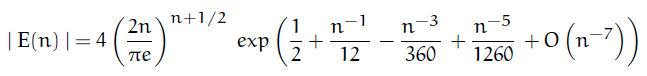
There is a standard asymptotic formula for the Euler numbers. For example at Mathworld or at the Digital Library of Mathematical Functions (NIST) (§24.11) one can find the formula one can find the formula
 |
The present author found two inclusions for the Euler numbers which appear to be new. They are reported on this page. The bounds given comprise a simple but amazingly efficient approximation to the Euler numbers which I will call the 'cute approximation'.
A sharp inclusion of the Euler numbers.
Let En denote the Euler numbers. If n is even and n ≥ 20 then
 |
For example the inclusion predicts
0.3887561841253070612..*10^2372 < |E(1000)| < 0.3887561841253070617..*10^2372.
And indeed |E(1000)| = 0.3887561841253070615..*10^2372.
Note that the factorial function is not referenced in these formulas.
A cute approximation of the Euler numbers.
The lower bound of the above inclusion can also be used as a convenient approximation for the Euler numbers. It then takes the form (assuming n even)
 |
Equivalently this formula can be stated as
 |
For example the standard approximation gives E(1000) ~ 0.38872..*10^2372, which amounts to 4 valid decimal numbers, whereas the last approximation gives for E(1000) an approximation with almost 18.2 valid decimal digits.
Asymptotic formulas
More generally let us look at three asymptotic formulas for the logarithm of the Euler numbers.
- LogE1(n) = (1/2+n)*ln(n)-(1/2+n)*ln(pi)+(5/2+n)*ln(2)-n
- LogE2(n) = (1/2+n)*ln(n)-(1/2+n)*ln(pi)+(5/2+n)*ln(2)-n*
(1-ln((120*n^2+9)/(120*n^2-1))) - LogE3(n) = (1/2+n)*ln(n)-(1/2+n)*ln(pi)+(5/2+n)*ln(2)-n*
(1-1/(12*n^2)*(1-1/(30*n^2)*(1-2/(7*n^2))))
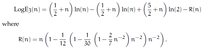 |
We see that formula 2 as well as formula 3 are refinements of formula 1. We are now focusing on formula 3 in its exponential form exp(LogE3(n)).
What makes this asymptotic approximation especially useful -- besides being a much better approximation than those given by the Digital Library of Mathematical Functions (see §24.11) -- is that the error of the approximation can be easily estimated.
In fact a convenient way to reason about the validity of an approximation formula is to give a lower bound for the number of exact decimal digits, i. e. to indicate the number of decimal digits which are guaranteed by the formula at least. In the case of exp(LogE3(n)) we have a good and simple way to express this bound:
EddE(n) = floor(3*log(3*n)) (valid for n ≥ 50).
For example for Euler(31622776) this bound says that 55 decimal digits of exp(logE3(n)) are guaranteed to be correct (the true value is 55.7).
To sum up: to compute an approximation to the Euler numbers E(n) with n ≥ 50 and n even compute exp(logE3(n)) and retain floor(3*log(3*n)) decimal digits of the result.
def EulerAsympt(n) :
    if n < 50 :
        print "Value error, n has to be ≥ 50"
        return
    if is_odd(n): return 0
    R = RealField(400)
    nn = n*n
    LogE = R((1/2+n)*ln(n)-(1/2+n)*ln(pi)+(5/2+n)*ln(2)
           -n*(1-1/(12*nn)*(1-1/(30*nn)*(1-2/(7*nn)))))
    E = (-1)^(n//2)*exp(LogE)
    Edd = 3*ln(3*n)
    print SciFormat(E, floor(Edd)-1)   # see SciFormat
    return E

for n in (49..52): print n, EulerAsympt(n)
   49 → Value error, n has to be ≥ 50
   50 → -6.0532852481886e54
   51 → 0
   52 → 6.50616248668461e57

EulerAsympt(31622776)
   8.569538850484365001271635684501232589197962270228803556e217235371
Note that the function displays only valid digits as we used this formatting function: SciFormat. With Sage the asymptotic formulas for the Euler numbers based on these formulas and the exact decimal digits (edd) of these approximations can be computed as follows.
AsyE1(n) = exp(LogE1(n))
AsyE2(n) = exp(LogE2(n))
AsyE3(n) = exp(LogE3(n))
EddE1(n) = -log10(abs(1-AsyE1(n)/abs(euler_number(n)))
EddE2(n) = -log10(abs(1-AsyE2(n)/abs(euler_number(n)))
EddE3(n) = -log10(abs(1-AsyE3(n)/abs(euler_number(n)))
EddEE(n) = floor(3*ln(3*n))
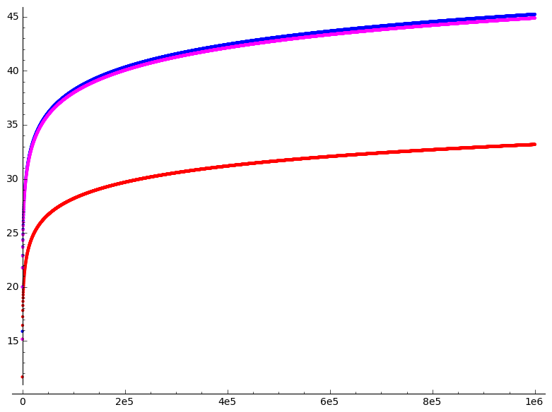
ANF = 50; END = 1000; STEP = 20
plot2 = list_plot([[n, EddE2(n)] for n in range(ANF,END,STEP)], color='red')
plot3 = list_plot([[n, EddE3(n)] for n in range(ANF,END,STEP)], color='blue')
plotE = list_plot([[n, EddEE(n)] for n in range(ANF,END,STEP)], color='magenta')
show(plot2 + plot3 + plotE)
The plot below compares the number of exact decimal digits of the approximation (formula 3, blue curve) with the number of exact decimal digits guaranteed by this formula, 3*ln(3*n) (magenta curve). For comparison the red curve shows the exact decimal digits of formula 3. Formula 1 (given by DLMF/NIST) gives a poor approximation not worth to be shown.
Restating exp(LogE3(n)) gives the following asymptotic expansion of the Euler number E(n) for n>0 even:
 |
Note: The 'cute approximation' was given on Jan. 21 2007 by the present author. Here the announcement in the newsgroup de.sci.mathematik. The inclusion was given on Jan. 22 2007, on this web page. Thanks to Achim Flammenkamp who drew my attention to an error in a previous version.
![]() Asymptotic inclusions and approximations for the Bernoulli numbers.
Asymptotic inclusions and approximations for the Bernoulli numbers.
![]() Asymptotic expansions of the factorial function.
Asymptotic expansions of the factorial function.