![]() To the Homepage of Factorial Algorithms
To the Homepage of Factorial Algorithms
Approximation Formulas
for the Factorial Function n!
Peter Luschny
We give an overview of approximations for the factorial function, convergent or asymptotic,
old or new, compare their efficiency and give hints for their application.
Although most formulas are variations of the asymptotic expansion of James Stirling (1692–1770)
we will reach a conclusion different from those given in most places. We will recommend
Stieltjes' formula whenever a numerical approximation of the factorial function is required.
The implementation for two of these formulas is given in pseudo-code below.
Some abbreviations:
kern0(n) = sqrt(2Pi/n)*(n/e)^n = kern2(n)/sqrt(n)
kern1(n) = sqrt(2Pi*n)*(n/e)^n = kern2(n)*sqrt(n)
kern2(n) = sqrt(2Pi)*(n/e)^n = sqrt(2Pi)*n^n*exp(-n)
kern0 - approximations
stieltjes0(n) : N=n+1; kern0(N)
stieltjes1(n) : N=n+1; kern0(N)*exp((1/12)/N)
stieltjes2(n) : N=n+1; kern0(N)*exp((1/12)/(N+(1/30)/N))
stieltjes3(n) : N=n+1; kern0(N)*exp((1/12)/(N+(1/30)/(N+(53/210)/N)))
stieltjes4(n) : N=n+1; kern0(N)*exp((1/12)/(N+(1/30)/(N+(53/210)/(N+(195/371)/N))))

henrici0(n)   : N=n+1; kern0(N)
henrici1(n)   : N=n+1; kern0(N)*exp(1/(12*N+1/N))
henrici2(n)   : N=n+1; kern0(N)*exp(5/2*1/(30*N+1/N))
henrici3(n)   : N=n+1; kern0(N)*exp((315*N-53/N)/(3780*N^2-510-53/N^2))

stirser0(n)   : N=n+1; kern0(N)
stirser1(n)   : N=n+1; kern0(N)*exp(1/(12*N))
stirser2(n)   : N=n+1; kern0(N)*exp(1/(12*N)*(1-1/(30*N^2)))
stirser3(n)   : N=n+1; kern0(N)*exp(1/(12*N)*(1-1/(30*N^2)*(1-2/(7*N^2))))
stirser4(n)   : N=n+1; kern0(N)*exp(1/(12*N)*(1-1/(30*N^2)*(1-2/(7*N^2)*(1-3/(4*N^2)))))
kern1 - approximations
ramanujan0(n):        kern1(n)
ramanujan1(n): N=2*n; kern1(n)*(1+1/N)^(1/6)
ramanujan2(n): N=2*n; kern1(n)*(1+1/N*(1+1/(2*N)))^(1/6)
ramanujan3(n): N=2*n; kern1(n)*(1+1/N*(1+1/(2*N)*(1+1/(15*N))))^(1/6)
ramanujan4(n): N=2*n; kern1(n)*(1+1/N*(1+1/(2*N)*(1+1/(15*N)*(1-11/(4*N)))))^(1/6)
ramanujan5(n): N=2*n; kern1(n)*(1+1/N*(1+1/(2*N)*(1+1/(15*N)*(1-1/(4*N)*(11-79/(7*N))))))^(1/6)

______ L0(n) :        kern1(n)
______ L1(n) : N=6*n; kern1(n)*(1+1/N)^(1/2)
______ L2(n) : N=6*n; kern1(n)*(1+1/N*(1+1/(2*N)))^(1/2)
______ L3(n) : N=6*n; kern1(n)*(1+1/N*(1+1/(2*N)*(1-31/(15*N))))^(1/2)
______ L4(n) : N=6*n; kern1(n)*(1+1/N*(1+1/(2*N)*(1-1/(15*N)*(31+139/(4*N)))))^(1/2)
______ L5(n) : N=6*n; kern1(n)*(1+1/N*(1+1/(2*N)*(1-1/(15*N)*(31+1/(4*N)*(139-9871/(7*N))))))^(1/2)

laplace0(n) :         kern1(n)
laplace1(n) : N=12*n; kern1(n)*(1+1/N)
laplace2(n) : N=12*n; kern1(n)*(1+1/N*(1+1/(2*N)))
laplace3(n) : N=12*n; kern1(n)*(1+1/N*(1+1/(2*N)*(1-139/(15*N))))
laplace4(n) : N=12*n; kern1(n)*(1+1/N*(1+1/(2*N)*(1-1/(15*N)*(139+571/(4*N)))))

nemes0(n)  :           kern1(n)
nemes1(n)  : N=12*n^2; kern1(n)*(1+1/N)^n
nemes2(n)  : N=12*n^2; kern1(n)*(1+1/N*(1+1/(10*N)))^n
nemes3(n)  : N=12*n^2; kern1(n)*(1+1/N*(1+1/(10*N)*(1+239/(21*N))))^n
nemes4(n)  : N=12*n^2; kern1(n)*(1+1/N*(1+1/(10*N)*(1+1/(21*N)*(239-46409/(20*N)))))^n

BuricElezovic0(n) :                kern1(n)
BuricElezovic1(n) :                kern1(n)*exp(1/(12*n))
BuricElezovic2(n) : N=1/(360*n^2); kern1(n)*exp(1/(12*n))*(1-N)^(1/n)
BuricElezovic3(n) : N=1/(360*n^2); kern1(n)*exp(1/(12*n))*(1-N*(1-(1447/14)*N))^(1/n)
BuricElezovic4(n) : N=1/(360*n^2); kern1(n)*exp(1/(12*n))*(1-N*(1-(1447/14)*N*(1-(1170727/4341)*N)))^(1/n)

nemesCF0(n) : kern1(n)
nemesCF1(n) : kern1(n)*(n/(n-1/12*1/n))^n
nemesCF2(n) : kern1(n)*(n/(n-1/12*1/(n+3/40*1/n)))^n
nemesCF3(n) : kern1(n)*(n/(n-1/12*1/(n+3/40*1/(n+2369/22680*1/n))))^n
nemesCF4(n) : kern1(n)*(n/(n-1/12*1/(n+3/40*1/(n+2369/22680*1/(n+7828759/10745784*1/n)))))^n

FengWang0(n): kern1(n)
FengWang1(n): kern1(n)*((n+1)/(n-1))^(1/24)
FengWang2(n): kern1(n)*((n+1)/(n-1))^((1/24)*(1-(11/30)/n^2))
FengWang3(n): kern1(n)*((n+1)/(n-1))^((1/24)*(1-(11/30)/n^2*(1+(43/231)/n^2)))
FengWang4(n): kern1(n)*((n+1)/(n-1))^((1/24)*(1-(11/30)/n^2*(1+(43/231)/n^2*(1+(1019/1290)/n^2))))
kern2 - approximations
demoivre0(n) : N=n+1/2; kern2(N)
demoivre1(n) : N=n+1/2; kern2(N)*(1-1/(24*N))
demoivre2(n) : N=n+1/2; kern2(N)*(1-1/(24*N)+1/(1152*N^2))
demoivre3(n) : N=n+1/2; kern2(N)*(1-1/(24*N)+1/(1152*N^2)+(1003/414720)/N^3)
demoivre4(n) : N=n+1/2; kern2(N)*(1-1/(24*N)+1/(1152*N^2)+(1003/414720)/N^3-(4027/39813120)/N^4)
demoivre5(n) : N=n+1/2; kern2(N)*(1-1/(24*N)+1/(1152*N^2)+(1003/414720)/N^3-(4027/39813120)/N^4
                                   -(5128423/6688604160)/N^5)

maclser0(n)  :          kern2(n+1/2)
maclser1(n)  : N=2*n+1; kern2(n+1/2)*exp(-1/(12*N))
maclser2(n)  : N=2*n+1; kern2(n+1/2)*exp(-1/(12*N)*(1-7/(30*N^2)))
maclser3(n)  : N=2*n+1; kern2(n+1/2)*exp(-1/(12*N)*(1-7/(30*N^2)*(1-62/(49*N^2))))
maclser4(n)  : N=2*n+1; kern2(n+1/2)*exp(-1/(12*N)*(1-7/(30*N^2)*(1-62/(49*N^2)*(1-381/(124*N^2)))))

wdsmith0(n)  : N=n+1/2; kern2(N)
wdsmith1(n)  : N=n+1/2; kern2(N)*exp((-1/24)/N)
wdsmith2(n)  : N=n+1/2; kern2(N)*exp((-1/24)/(N+(7/120)/N))
wdsmith3(n)  : N=n+1/2; kern2(N)*exp((-1/24)/(N+(7/120)/(N+(1517/5880)/N)))
wdsmith4(n)  : N=n+1/2; kern2(N)*exp((-1/24)/(N+(7/120)/(N+(1517/5880)/(N+(164715/297332)/N))))

cantrell0(n) : N=n+1/2; kern2(N)
cantrell1(n) : N=n+1/2; kern2(N)/(1+1/(24*N-1/2))
cantrell2(n) : N=n+1/2; kern2(N)/(1+1/(24*N-1/2+1/((1440/2021)*N)))
cantrell3(n) : N=n+1/2; kern2(N)/(1+1/(24*N-1/2+1/((1440/2021)*N+1/((686186088/125896643)*N))))
cantrell4(n) : N=n+1/2; kern2(N)/(1+1/(24*N-1/2+1/((1440/2021)*N+1/((686186088/125896643)*N
                                   +1/((1521596612992267104/4596084813365743279)*N)))))

lanczos0(n)  : N=n+1/2; kern2(N)
lanczos1(n)  : N=n+1/2; kern2(N)*(1-(1/24)*(1/(n+1)))
lanczos2(n)  : N=n+1/2; kern2(N)*(1-(1/24)*(1/(n+1))-(23/1152)*(1/((n+1)*(n+2))))
lanczos3(n)  : N=n+1/2; kern2(N)*(1-(1/24)*(1/(n+1))-(23/1152)*(1/((n+1)*(n+2)))
                                   -(11237/414720)*(1/((n+1)*(n+2)*(n+3))))

wehmeier0(n) : kern2(n)*sqrt(n)
wehmeier1(n) : kern2(n)*sqrt(n+1/6)
wehmeier2(n) : kern2(n)*sqrt(n+1/6+(1/72)/n)
wehmeier3(n) : kern2(n)*sqrt(n+1/6+(1/72)/n-(31/6480)/n^2)
wehmeier4(n) : kern2(n)*sqrt(n+1/6+(1/72)/n-(31/6480)/n^2-(139/155520)/n^3)

gosper0(n)   : kern2(n)*sqrt(n)
gosper1(n)   : kern2(n)*sqrt(n+1/6)
gosper2(n)   : kern2(n)*sqrt(n+1/6)*(1+(1/144)/n^2)
gosper3(n)   : kern2(n)*sqrt(n+1/6)*(1+(1/144)/n^2-(23/6480)/n^3)
gosper4(n)   : kern2(n)*sqrt(n+1/6)*(1+(1/144)/n^2-(23/6480)/n^3+(5/41472)/n^4)
gosper5(n)   : kern2(n)*sqrt(n+1/6)*(1+(1/144)/n^2-(23/6480)/n^3+(5/41472)/n^4+(4939/6531840)/n^5)

nemesG1(n)   : N=n+1/4; kern2(n)*sqrt(n+1/6)
nemesG2(n)   : N=n+1/4; kern2(n)*sqrt(n+1/6)*(1+(1/144)/N^2)
nemesG3(n)   : N=n+1/4; kern2(n)*sqrt(n+1/6)*(1+(1/144)/N^2-(1/12960)/N^3)
nemesG4(n)   : N=n+1/4; kern2(n)*sqrt(n+1/6)*(1+(1/144)/N^2-(1/12960)/N^3-(257/207360)/N^4)
nemesG5(n)   : N=n+1/4; kern2(n)*sqrt(n+1/6)*(1+(1/144)/N^2-(1/12960)/N^3-(257/207360)/N^4-(53/2612736)/N^5)
nemesG6(n)   : N=n+1/4; kern2(n)*sqrt(n+1/6)*(1+(1/144)/N^2-(1/12960)/N^3-(257/207360)/N^4-(53/2612736)/N^5
                                               +(5741173/9405849600)/N^6)

gospersmith0(n): N=n+1/2; NN=N^2; sqrt(2*Pi)*exp(-N)*(NN)^(N/2)
gospersmith1(n): N=n+1/2; NN=N^2; sqrt(2*Pi)*exp(-N)*(NN-(1/12))^(N/2)
gospersmith2(n): N=n+1/2; NN=N^2; sqrt(2*Pi)*exp(-N)*(NN+(1/12)*(-1+(1/(10*NN))))^(N/2)
gospersmith3(n): N=n+1/2; NN=N^2; sqrt(2*Pi)*exp(-N)*(NN+(1/12)*(-1+(1/(10*NN))*(1-(185/(756*NN)))))^(N/2)

luschny0(n): N=n+1/2; NN=24*N^2; kern2(N)
luschny1(n): N=n+1/2; NN=24*N^2; kern2(N)*(1-1/NN)^N
luschny2(n): N=n+1/2; NN=24*N^2; kern2(N)*(1-1/NN*(1-19/(10*NN)))^N
luschny3(n): N=n+1/2; NN=24*N^2; kern2(N)*(1-1/NN*(1-1/(10*NN)*(19-2561/(21*NN))))^N
luschny4(n): N=n+1/2; NN=24*N^2; kern2(N)*(1-1/NN*(1-1/(10*NN)*(19-1/(21*NN)*(2561-874831/(20*NN)))))^N

luschnyCF0(n): N=n+1/2; kern2(N)
luschnyCF1(n): N=n+1/2; kern2(N)*(N/(N+1/24*1/N))^N
luschnyCF2(n): N=n+1/2; kern2(N)*(N/(N+1/24*1/(N+3/80*1/N)))^N
luschnyCF3(n): N=n+1/2; kern2(N)*(N/(N+1/24*1/(N+3/80*1/(N+18029/45360*1/N))))^N
luschnyCF4(n): N=n+1/2; kern2(N)*(N/(N+1/24*1/(N+3/80*1/(N+18029/45360*1/(N+6272051/14869008*1/N)))))^N
miscellaneous approximations
maclstir0(n) : (  2*maclser0(n)+    stirser0(n))/3
maclstir1(n) : ( 32*maclser1(n)+ 31*stirser1(n))/63
maclstir2(n) : ( 64*maclser2(n)+ 63*stirser2(n))/127
maclstir3(n) : (128*maclser3(n)+127*stirser3(n))/255

windschitl(n): N=n+1;   sqrt(2*Pi/N)*((N/e)*sqrt(N*sinh(1/N)))^N
wdsmith*(n)  : N=n+1/2; sqrt(2*Pi)*((N/e)*sqrt(2*N*tanh(1/(2*N))))^N

nemes*(n)    : N=n;     sqrt(2*Pi*N)*((N+1/(12*N-1/(10*N)))/e)^N
nemesgam(n)  : N=n+1;   sqrt(2*Pi/N)*((N+1/(12*N-1/(10*N)))/e)^N
luschny*(n)  : N=n+1/2; sqrt(2*Pi)*((N-1/(24*N+19/(10*N)))/e)^N
A popular formula (but not recommended)
Digits := 20;
lanczos7 :=  proc(z) local x, t, p;
p := [0.99999999999980993, 676.5203681218851, -1259.1392167224028,
 771.32342877765313, -176.61502916214059, 12.507343278686905,
-0.13857109526572012, 9.9843695780195716e-6, 1.5056327351493116e-7];

x := p[1]+p[2]/(z+1)+p[3]/(z+2)+p[4]/(z+3)+p[5]/(z+4)+
     p[6]/(z+5)+p[7]/(z+6)+p[8]/(z+7)+p[9]/(z+8);

t := z+7.5; sqrt(2*Pi)*t^(z+0.5)*exp(-t)*x end:
This formula, due to Lanczos, is popular presumably because it was included in the 'Numerical Recipes in C' book in the early 1990. Why it is not recommended (at least not for the real domain) can be seen from this little test computing 100!, 1000! and 10000!. It shows the number of exact decimal digits.
| n | 100 | 1000 | 10000 |
| exact decimal digits | 13.2 | 12.8 | 12.7 |
A simple new formula (recommended)
Digits := 50;
luschnyCF4 := proc(n) local c, N, p, logF; N := n + 1/2;
c := array(0..4, [1/24, 3/80, 18029/45360, 6272051/14869008]);
p := N^2/(N+c[0]/(N+c[1]/(N+c[2]/(N+c[3]/N))));
logF := ln(2*Pi)/2 + N*(ln(p)-1);
return exp(logF) end:
The same test applied to this formula shows the new formula is far more than a match for the Lanczos formula. The formula is due to the present writer.
| n | 100 | 1000 | 10000 |
| exact decimal digits | 21.5 | 30.5 | 39.5 |
A numerical example
To give an idea how this formula works numerically we show the successive approximations to 100!. At the left hand margin the number of exact decimal digits are displayed (with our sign convention).
How well do these formulas perform?
We now look at the general case. The following table displays the number of exact decimal digits (edd) of all the formulas above for some values of n. Exact decimal digits are defined as -log10(abs(1-approximation/trueValue)). log10 denotes the logarithm to the base 10.
edd(n) = -log10(abs(1 - approximation(n) / n!)).
In the following table the i-th entry (i=0,1,2,... from the left hand side to the
right hand side) in a line starting with 'name' is the edd of formula name(i)(n).
The '-' sign indicates that the approximation is smaller and the '+' sign (not
displayed) indicates that the approximation is larger than the true value.
For example we see from the table that formula nemes1 gives the same number of
exact decimal digits as the formula ramanujan2.
---------------------------------------------------------------------------------------
Formula          n!               exact decimal digits, edd(n)
---------------------------------------------------------------------------------------

Laplace      00100!   -3.1   -6.5    8.6   11.7  -13.1    16.2    17.2   -20.4   -21.1
De Moivre    00100!    3.4   -7.1   -8.6   12.0   13.1   -16.4   -17.2    20.5   -22.8
NemesG       00100!          -6.2   10.1   10.9  -14.9   -15.2    19.4    19.2   -23.0

Gosper       00100!   -3.1   -6.2    8.5  -11.9   13.1    17.5    17.2    21.2    21.1
Wehmeier     00100!   -3.1   -6.2    8.6   11.4  -13.1   -15.9    17.2   -20.0   -21.1
Ramanujan    00100!   -3.1   -5.7   -9.2   11.0  -13.3   -15.4    17.3    19.5   -21.1

Nemes        00100!   -3.1          -9.2         -13.2            17.3           -21.1
Luschny      00100!    3.4          -8.5          13.1           -17.2            21.1
Henrici      00100!   -3.1          -8.4         -13.2            17.2
GosperSonin  00100!    3.4          -8.4          13.0           -17.2
MaclSeries   00100!    3.4          -8.6          13.1           -17.2            21.1
StirSeries   00100!   -3.1           8.6         -13.1            17.3           -21.1
BuricElezovic  100!   -3.1           8.6         -13.1            17.2           -21.1
FengWang     00100!   -3.1           7.5          12.2            16.3            20.8

NemesCF      00100!    3.1           8.2          13.2            17.3            21.5
W.D.Smith    00100!    3.4          -8.6          13.2           -17.5            21.5
Cantrell     00100!    3.4          -8.6          13.2           -17.5            21.5
Stieltjes    00100!   -3.1           8.6         -13.2            17.5           -21.5
LuschnyCF    00100!    3.4          -8.8          13.2           -17.6            21.5

Lanczos7     00100!                              -13.2
Windschitl   00100!                              -13.2
W.D.Smith*   00100!                               13.2
Nemes*       00100!                              -13.2
NemesGamma   00100!                              -13.2
Luschny*     00100!                               13.2
---------------------------------------------------------------------------------------
Laplace      01000!   -4.1   -8.5   11.6   15.6  -18.1    22.2    24.2   -28.3   -30.1
De Moivre    01000!    4.4   -9.1  -11.6   16.0   18.1   -22.4   -24.3    28.6   -29.1
NemesG       01000!          -8.2   13.1   14.9  -19.7   -21.2    26.9    27.2   -33.5

Gosper       01000!   -4.1   -8.2   11.4  -15.9   18.1    23.1    24.2    29.7    30.1
Wehmeier     01000!   -4.1   -8.2   11.6   15.4  -18.1   -21.9    24.2   -28.0   -30.1
Ramanujan    01000!   -4.1   -7.7  -12.2   15.0  -18.3   -21.4    24.3    27.5   -30.1

Nemes        01000!   -4.1         -12.2         -18.2            24.3           -30.1
Luschny      01000!    4.4         -11.5          18.1           -24.2            30.1
Henrici      01000!   -4.1         -11.4         -18.2            24.2
GosperSonin  01000!    4.4         -11.4          18.0           -24.2
MaclSeries   01000!    4.4         -11.6          18.1           -24.2            30.1
StirSeries   01000!   -4.1          11.6         -18.1            24.2           -30.1
BuricElezovic 1000!   -4.1          11.6         -18.1            24.2           -30.1
FengWang     01000!   -4.1          10.5          17.2            23.3            29.8

NemesCF      01000!    4.1          11.2          18.2            24.3            30.5
W.D.Smith    01000!    4.4         -11.6          18.2           -24.5            30.5
Cantrell     01000!    4.4         -11.6          18.2           -24.5            30.5
Stieltjes    01000!   -4.1          11.6         -18.2            24.4           -30.4
LuschnyCF    01000!    4.4         -11.8          18.2           -24.6            30.5

Lanczos7     01000!                -12.8
Windschitl   01000!                              -18.2
W.D.Smith*   01000!                               18.2
Nemes*       01000!                              -18.2
NemesGamma   01000!                              -18.2
Luschny*     01000!                               18.2
---------------------------------------------------------------------------------------
Laplace      10000!   -5.1  -10.5   14.6   19.6  -23.1    28.2    31.2   -36.3   -39.1
De Moivre    10000!    5.4  -11.1  -14.6   20.0   23.1   -28.5   -31.2    36.6   -37.1
NemesG       10000!         -10.2   16.1   18.9  -24.7   -27.2    33.7    35.2   -42.1

Gosper       10000!   -5.1  -10.2   14.4  -19.9   23.1    29.1    31.2    37.6    39.1
Wehmeier     10000!   -5.1  -10.2   14.6   19.3  -23.1   -27.9    31.2   -36.0   -39.1
Ramanujan    10000!   -5.1   -9.7  -15.2   19.0  -23.3   -27.4    31.3    35.5   -39.1

Nemes        10000!   -5.1         -15.2         -23.2            31.3           -39.1
Luschny      10000!    5.4         -14.5          23.1           -31.2            39.1
Henrici      10000!   -5.1         -14.4         -23.2            31.2
GosperSonin  10000!    5.4         -14.4          23.0           -31.2
MaclSeries   10000!    5.4         -14.6          23.1           -31.2            39.1
StirSeries   10000!   -5.1          14.6         -23.1            31.2           -39.1
BuricElezovic 10000!  -5.1          14.6         -23.1            31.2           -39.1
FengWang     10000!   -5.1          13.5          22.2            30.3            38.8

NemesCF      10000!    5.1          14.2          23.2            31.3            39.5
W.D.Smith    10000!    5.4         -14.6          23.2           -31.5            39.5
Cantrell     10000!    5.4         -14.6          23.2           -31.5            39.5
Stieltjes    10000!   -5.1          14.6         -23.2            31.4           -39.4
LuschnyCF    10000!    5.4         -14.8          23.2           -31.6            39.5

Lanczos7     10000!         -12.7
Windschitl   10000!                              -23.2
W.D.Smith*   10000!                               23.2
Nemes*       10000!                              -23.2
NemesGamma   10000!                              -23.2
Luschny*     10000!                               23.2
Exact digits and efficiency
Note that the above table is misleading in one respect: It shows only the exact decimal digits of a formula; however it does not to give evidence for efficiency. Although the asymptotic even Nemes formulas nemesG2, nemesG4, etc., the odd De Moivre formulas demoivre1, demoivre3 and the odd Gosper formulas gosper5, gosper7 score highest in the respective columns they are not the most efficient ones. The most efficient ones are the continued fraction formulas (distinguished by color (blue and purple) in the table).
To illustrate the last remark we give a 'nemesG' formula in a form which has a comparable amount of computational cost as the simple new formula recommended above.
Digits:= 30;
nemesG5 := proc(x) local X, G, S, n; X := x + 1/4;
G := array(0..4, [1/144,-1/12960,-257/207360,-53/2612736]);
S := 1 + G[0]/X^2 + G[1]/X^3 + G[2]/X^4 + G[3]/X^5;
return x^x*exp(-x)*sqrt(2*Pi*(x+1/6))*S end:
The test applied to this formula shows that the new formula 'LuschnyCF' is far more efficient than the 'NemesG' formula.
| Formula | n | 100 | 1000 | 10000 |
| NemesG5 | edd | 14.9 | 19.7 | 24.7 |
| LuschnyCF4 | edd | 21.5 | 30.5 | 39.5 |
| StirlingSeries4 | edd | 21.1 | 30.1 | 39.1 |
With regard to the ratio (exact decimal digits) / (computational cost) the popular 'Lanczos7' is perhaps the most inefficient formula shown on this page.
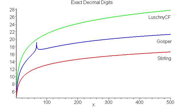
The plot below compares on a continuous scale the exact decimal digits of the Stirling and the Gosper formula with the Luschny-CF formula. The peak in the blue edd-function is due to the fact that the Gosper5 formula is exact at x = 67.0033148435486248...
Which approximation to choose?
The formulas given are mostly asymptotic formulas and this means they only give good approximations
if x is large. However, for small values of x there is a simple trick to overcome this shortcoming at
no great cost. Shift x in the direction → +∞ before evaluating and divide by the shifted amount afterwards.
This is, of course, nothing else but a clever application of the functional equation of x!.
I am quite fond of the continued fraction approximation of T. J. Stieltjes because of its simplicity and the small constants
involved. Note especially that this is a convergent approximation! So I built the above-mentioned trick in the
following simple function based on the stieltjes3 formula and recommend its use if only moderate precision is needed.
Stieltjes3Factorial(x)
y = x+1; p = 1;
while y < 7 do p = p*y; y = y+1; od;
r = exp(y*log(y)-y + 1/(12*y+2/(5*y+53/(42*y))));
if x < 7 then r = r/p fi;
return r*sqrt(2*Pi / y) end;
This approximation guarantees 9 valid decimal digits. And you can expect about 7/2+3*log(x) valid significant
decimal digits for x>=10. For programming a pocket calculator the following simplification
of the fourth line is even better suited:
r = exp(y*(log(y)-1)+1/(2*(6*y+1/(5*(y+1/(4*y))))));
In the following plot the blue line represents the guaranteed 9 decimal digits, the
green zigzag line shows the effect of the shift/divide-trick, and the red curve is the number of exact
decimal digits of the 'pure' stieltjes3 approximation.
How to display approximation values?
It is good practice to display only the valid digits of an approximation and not to leave the user more
or less helplessly looking at long strings of digits figuring out how much of these digits he might assume as valid.
However, how this is done depends much on the implementation language. I give an example using pseudo-Maple-style,
which in turn uses a formatting scheme which is very similar to the one used in the computer language 'C'.
PrintFactorial(x)
# Number of valid significant decimal digits for StieltjesFactorial.
l = floor(7/2+3*log(x));
# Put formatting specifications in the format string.
format = sprintf("%d! = %s%de\n",x,"%1.",l-1);
# Add some internal guarding digits and evaluate.
F = evalf(Stieltjes3Factorial(x),l+6);
printf(format, F) end;
Using this special print function to display the approximations to (2^i)!
Sequence( PrintFactorial(2^i), i = 0..12);
gives the following output, which shows only valid digits (the last digit might be rounded).
   1! = 1.00e+00
   2! = 2.0000e+00
   4! = 2.400000e+01
   8! = 4.03200000e+04
  16! = 2.0922789888e+13
  32! = 2.631308369337e+35
  64! = 1.26886932185884e+89
 128! = 3.85620482362580422e+215
 256! = 8.5781777534284265412e+506
 512! = 3.477289793132605363283e+1166
1024! = 5.41852879605885728307692e+2639
2048! = 1.6726919319100117051699525e+5894
4096! = 3.642736389457041931565827470e+13019
A higher precision approximation
... and now we are going for the Big Pizza. The next approximation guarantees 16 valid decimal digits.
And you can expect about 5/2+(13/2)*log(x) valid significant decimal digits for x >= 10 (see the next figure).
I just give the pseudo-code because things are very similar to the things explained in the last two sections.
However, there is a small difference. This time we make explicit that we are using the logarithmic version of
the continued fraction formula. This gives an additional layer of flexibility.
|
StieltjesLnFactorial(z) a0 = 1/12; a1 = 1/30; a2 = 53/210; a3 = 195/371; a4 = 22999/22737; a5 = 29944523/19733142; a6 = 109535241009/48264275462; Z = z+1; (1/2)*ln(2*Pi)+(Z-1/2)*ln(Z)-Z + a0/(Z+a1/(Z+a2/(Z+a3/(Z+a4/(Z+a5/(Z+a6/Z)))))) end; StieltjesFactorial(x) y = x; p = 1; while y < 8 do p = p*y; y = y+1; od; r = exp(StieltjesLnFactorial(y)); if x < 8 then r = (r*x)/(p*y) fi; r end; |
PrintFactorial(x)
l = floor((5+13*log(x))/2);
format = sprintf("%d! = %s%de\n",x,"%1.",l-1);
F = evalf(StieltjesFactorial(x),l+6);
printf(format, F) end;
   1! = 1.00e+00
   2! = 2.000000e+00
   4! = 2.4000000000e+01
   8! = 4.032000000000000e+04
  16! = 2.0922789888000000000e+13
  32! = 2.631308369336935301672180e+35
  64! = 1.2688693218588416410343338934e+89
 128! = 3.856204823625804217356770659234637e+215
 256! = 8.5781777534284265411908227168123262516e+506
 512! = 3.477289793132605363283045917545604711992251e+1166
1024! = 5.4185287960588572830769219446838547380015539636e+2639
2048! = 1.672691931910011705169952468793676234018507002356737e+5894
4096! = 3.6427363894570419315658274703116469205712449235098554300e+13019

The 100 digits challenge:
Using Stieltjes' CF for unlimited precision
Approximations like the Stirling or the De Moivre or the Nemes approximations are asymptotic in their character. They do not converge to the true value. On the other hand the continued fraction developments of Stieltjes or Cantrell or Luschny do converge. The asymptotic developments are fine if you work with fixed length arithmetic. For instance if you have to work with standard formats of computer languages like 'float' or 'double' it is easy to find a formula which is appropriate for these types in the table above and that's it. (Well, a careful implementation taking the rounding error into account is still needed, of course.) However, increasingly often applications demand higher precision and assuming that your computing environment supports unlimited arithmetic we can implement also these continued fraction algorithms without pain.
Just to keep things simple and concrete let us pose the 100 digits question. Suppose I want to approximate 100! (which has 158 decimal digits) to 100 decimal digits. How can I proceed? We stay with our favorite convergent approximation, the Stieltjes continued fractions. First we have to compute all the constants involved. This is far from being trivial. Stieltjes himself groaned about it: "Le calcul est trés pénible ... la loi de ces nombres paraît extrêmement compliqué". Using the algorithms of Rutishauser and Akiyama-Tanigawa we can compute nowadays the coefficients much more easily than Stieltjes could:
StieltjesCF := proc(len)
local s, m, n, k, a, b, c, AkiyamaTanigawa;

# Computes Bernoulli(2*p+2)/((2*p+1)*(2*p+2))
# using the Akiyama-Tanigawa algorithm

AkiyamaTanigawa := proc(l) local a,t,n,m,j,k;
n := 2*l+1; t := array(1..n); a := array(1..l);
t[1] := 1; k := 1;
for m from 2 to n do
  t[m] := 1/m;
  for j from m-1 by -1 to 1 do
    t[j] := j*(t[j]-t[j+1]);
  od;
  if type(m,odd) then
     a[k] := (-1)^(k+1)*t[1]/((2*k-1)*(2*k));
     k := k+1;
  fi;
od;
a end:

# Computes the Stieltjes continued fraction for the
# Gamma function using Rutishauser's QD-algorithm.

s := AkiyamaTanigawa(len);
m := array(1..len,1..len):
for n to len   do m[n,1] := 0 od;
for n to len-1 do m[n,2] := s[n+1]/s[n] od;
for k from 3 to len do
  for n to len-k+1 do
    a := m[n+1,k-2]; b := m[n+1,k-1]; c := m[n,k-1];
    m[n,k] := `if`(type(k,odd), a+b-c, a*b/c);
  od;
od;
m[1,1] := s[1]; [seq(m[1,k],k=1..len)] end:

# Example call
StieltjesCF(6);
[1/12, 1/30, 53/210, 195/371, 22999/22737]
Having found a way to compute the constants it is easy now to finish the job and compute Stieltjes approximations for n! to any order we whish.
Stieltjes := proc(n, ord) local N, c, q, i;
N := n + 1; q := N;
c := StieltjesCF(ord);
for i from ord by -1 to 2 do
    q := N + c[i] / q od;
sqrt(2*Pi/N)*(N/exp(1))^N*exp(1/(12*q))
end:
In our example (and using Maple) we can now call 'Stieltjes(n, 32); evalf(%, 100)' for n = 100. For comparison the first value given below is evalf(n!, 100) and the second value is the approximation. ('evalf(x, 100)' here means that we want to compute the floating point value of x to 100 digits.)
0.9332621544394415268169923885626670049071596826438162146859296389521759999322991560894146397615651829*10^158
0.9332621544394415268169923885626670049071596826438162146859296389521759999322991560894146397615651976*10^158
We see that the first 97 decimal digits are exact; so we learned that it is always a good idea to compute with some extra digits (say 100+5 in our case) to compensate for the rounding error.
The computation of the Laplace-coefficients
Laplace's approximation is a famous approximation to the factorial function — for historic reasons. Here we have found no reasons to use this formula. Nevertheless we show how to compute the coefficients of the Laplace formula.
h := proc(k) option remember; local j;
`if`(k=0,1,(h(k-1)/k-add((h(k-j)*h(j))/(j+1),j=1..k-1))/(1+1/(k+1))) end:

coeffLaplace := proc(n) option remember;
h(2*n)*2^n*pochhammer(1/2,n) end:
The computation of the 'de Moivre'-coefficients
This is amazingly simple, provided you already have the Bernoulli numbers. (If not, use the Akiyama-Tanigawa algorithm given above.) Here is a Maple implementation:
G := proc(n) option remember; local j, R;
R := seq(2*j, j = 1 .. iquo(n+1,2));
`if`(n=0,1,add(bernoulli(j,1/2)*G(n-j+1)/(n*j),j=R)) end:
The relationship between these coefficients and the Bernoulli numbers are due to De Moivre, 1730, which of course also explains the name of the formula. 281 years old but still better than those "ultimate extremely accurate formulas" of Mortici.
The computation of the Lanczos-coefficients
C. Lanczos, A precision approximation of the gamma function, J. SIAM Numer. Anal., Ser. B, 1 (1964), 86-96.
Here we look at formula (21) on page 90. A Maple implementation:
Lanczos := proc(n) exp(1+LambertW((x^2-1)/exp(1)));
coeftayl(taylor(%,x=0,2*n+2),x=0,2*n+1);
simplify(-%*(2*n+1)*pochhammer(1/2,n)/sqrt(2),exp) end:
The computation of the 'NemesG'-coefficients
[Now some fiction, also a puzzle: The mysterious J-function.] One day, while studying -- no, not Mortici but Y. L. Luke's treatise -- Gery saw the beautiful expansion given at the top of this page (in fact the formula on this page is by a hairbreadth better). "Wow" he thought, "I'd like to have also such a nice formula for the factorial." So what was important was to find a way to mimic the even expansion from Luke's book, which is due to J. L. Fields (A note on the asymptotic expansion of a ratio of gamma functions. Proc. Edinburgh Math. Soc., 15:43–45, 1966.) This means he had to look for a sequence of even polynomials. Well, after some hard thinking Gery came up with these polynomials:
G := proc(n,x) local j;
add(x^(2*j)*2^j*6^(j-n)*GAMMA(1/2+j)/(GAMMA(n-j+1)*GAMMA(1/2+j-n)),j=0..n)-
add(G(j,x)*(-4)^(j-n)*(GAMMA(n)/(GAMMA(n-j+1)*GAMMA(j))),j=1..n-1);
sort(%) end:

for i from 0 to 5 do G(i,x)*24^i od;

                                  1
                              24 x^2  - 2
                         1728 x^4  + 96 x^2  - 6
                  207360 x^6  + 17280 x^4  + 432 x^2  - 20
         34836480 x^8  + 3317760 x^6  + 134784 x^4  + 2112 x^2  - 74
7524679680*x^10 + 766402560*x^8 + 36080640*x^6 + 960768*x^4 + 10896*x^2 - 300
At this moment an email from James S. arrived announcing a totally mysterious function. James wrote: "Dear Gery, please look at this convolved function. Can you make any sense out of it?"
J := proc(k) option remember; local j;
`if`(k=0,1,(J(k-1)/k-add((J(k-j)*J(j))/(j+1),j=1..k-1))/(1+1/(k+1))) end:
Gery again thought hard but this time he could not make any sense with this function. However, his just discovered polynomials still were on his desktop and he decided to play just for fun the umbral game. This means to replace x^i by a function call x(i). Well, so he evaluated his polynomials with J(i) in lieu of x^i. And here is what he saw:
seq(subs({seq(x^i=J(i), i=0..degree(G(k,x),x))}, G(k,x)),k=0..7);

            1    -1     -257     -53     5741173       37529
     1, 0, ---, -----, ------, -------, ----------, -----------, ...
           144  12960  207360  2612736  9405849600  18811699200
Conclusions and Recommendations
The Stirling formula is a useful formula when we have to do some Big-O
(complexity-) analysis. But if we are only interested in the numerical
evaluation of the factorial function then there is no reason to use the Stirling approximation or some
of its many asymptotic variants. Because there exist convergent approximations which are
- computational as simple as the Stirling formula,
- computational more efficient then the Stirling formula,
- and can equally well be used in the context where only a simple estimate is required or in a context where an arbitrary precision computation is required.
In our judgement there are three outstanding formulas which we declare the winners of our little contest.
- The continued fraction formula of Thomas J. Stieltjes.
- The continued fraction 'half-shift' formula of Warren D. Smith.
- The continued fraction formula of Peter Luschny (luschnyCF).
Clearly the continued fraction of W. D. Smith is a variant of Stieltjes' formula. And the coefficients
of this formula are slightly larger than those of the Stieltjes formula. Another
runner-up is Cantrell's formula, which is numerically on par with Smith's
formula but has even larger rational constants (which does not really matter if
we are using floating point arithmetic with fixed precision). Note that we
looked only at the real range x > 1. If considered throughout the complex half-plane Re(z)
> 1 there might be some special strength or weakness in the formulas which we
have not noticed.
Summa summarum we recommend Stieltjes's CF-formula or Luschny's CF-formula whenever a numerical approximation of the
factorial function is required.
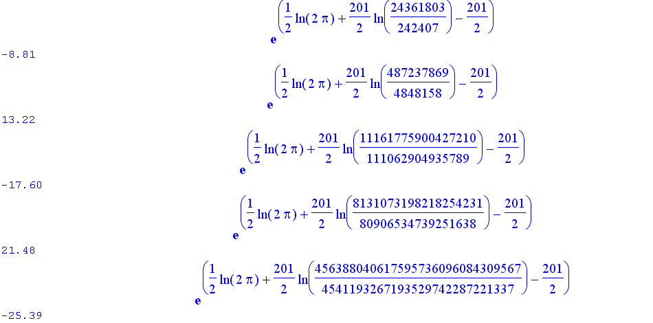
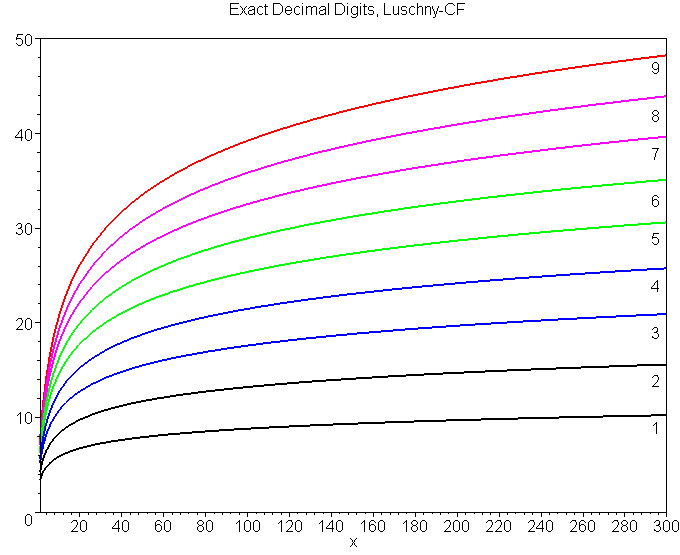
S * H * O * W * D * O * W * N
| StieltjesCF | LuschnyCF | StieltjesCF | LuschnyCF | StieltjesCF | LuschnyCF | |||
| n | 100 | 1000 | 10000 | |||||
| 1 | 8.57 | -8.81 | 11.56 | -11.81 | 14.56 | -14.81 | ||
| 2 | -13.18 | 13.22 | -18.16 | 18.21 | -23.15 | 23.21 | ||
| 3 | 17.46 | -17.60 | 24.44 | -24.58 | 31.43 | -31.58 | ||
| 4 | -21.47 | 21.48 | -30.43 | 30.46 | -39.43 | 39.46 | ||
| 5 | 25.30 | -25.39 | 36.25 | -36.37 | 47.25 | -47.36 | ||
| 6 | -28.95 | 28.94 | -41.90 | 41.92 | -54.89 | 54.91 | ||
| 7 | 32.48 | -32.55 | 47.42 | -47.52 | 62.41 | -62.51 | ||
| 8 | -35.88 | 35.86 | -52.82 | 52.83 | -69.81 | 69.83 | ||
| 9 | 39.19 | -39.25 | 58.12 | -58.21 | 77.11 | -77.20 | ||
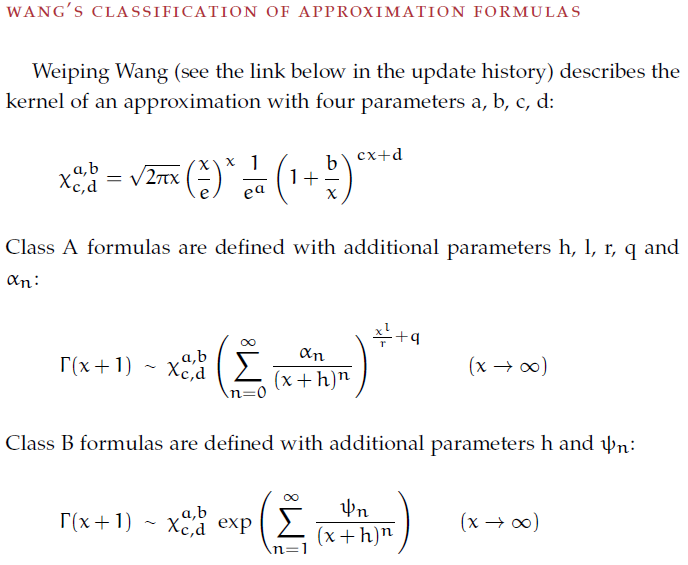
| Example formulas in the Wang classification. | |||||||||
| Type | Reference | a | b | c | d | h | l | q | r |
| A | Laplace | 0 | 0 | - | - | 0 | 0 | 0 | 1 |
| A | Wehmeier | 0 | 0 | - | - | 0 | 0 | 0 | 2 |
| A | Batir | 0 | 0 | - | - | 0 | 0 | 0 | 4 |
| A | Ramanujan | 0 | 0 | - | - | 0 | 0 | 0 | 6 |
| A | Chen-Lu-Wang | 0 | 0 | - | - | 0 | 0 | 0 | r |
| A | Nemes | 0 | 0 | - | - | 0 | 1 | 0 | 1 |
| A | Nemes | 0 | 0 | - | - | 0 | 1 | 0 | 4/5 |
| A | Chen | 0 | 0 | - | - | 0 | 1 | 0 | 2 |
| A | Chen-Lin | 0 | 0 | - | - | 0 | l | 0 | r |
| A | Mortici | a | a | 1 | 0 | 0 | 0 | 0 | 6 |
| A | Lu | 1/2 | 1/2 | 1 | 1/2 | 0 | 0 | 0 | r |
| A | Chen-Liu | a | a | 1 | d | 0 | 0 | 0 | r |
| A | De Moivre | 1/2 | 1/2 | 1 | 1/2 | 1/2 | 0 | 0 | 1 |
| A | Gosper | 0 | 1/6 | 0 | 1/2 | 0 | 0 | 0 | 1 |
| A | Nemes | 1/2 | 1/6 | 0 | 1/2 | 1/4 | 0 | 0 | 1 |
| A | Luschny | 1/2 | 1/2 | 1 | 1/2 | 1/2 | 1 | 1/2 | 1 |
| A | Gosper-Smith | 1/2 | 1/2 | 1 | 1/2 | 1/2 | 1 | 1/4 | 2 |
| A | Paris | 1/2 | 1/2 | 1 | 1/2 | 1/2 | 1 | 1/6 | 3 |
| A | Paris | 1/2 | 1/2 | 1 | 1/2 | 1/2 | 1 | 1/8 | 4 |
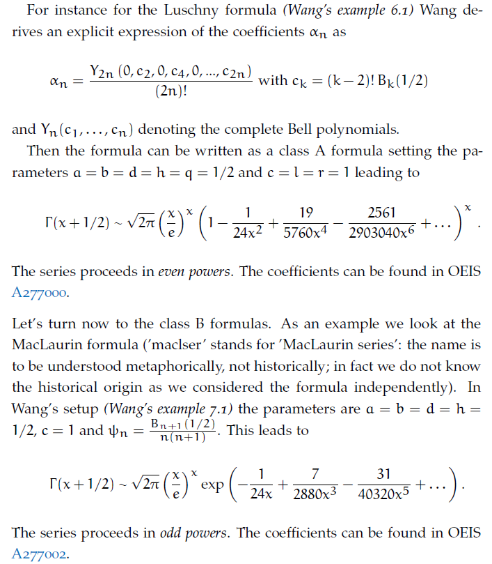
| B | MacLaurin | 1/2 | 1/2 | 1 | 1/2 | 1/2 | - | - | - |
| B | Batir | 0 | 1/2 | 0 | 1/2 | 3/8 | - | - | - |
| B | Mortici | a | a | 1 | 1/2 | 0 | - | - | - |
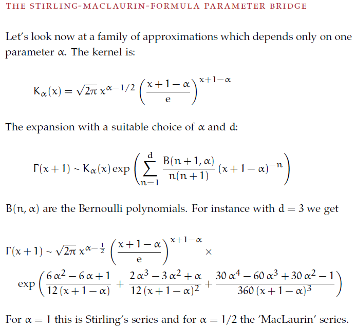
Maple
StirMaclSer := proc(alpha,x,d) local kern, C, X:
X := x + 1 - alpha;
kern := sqrt(2*Pi)*x^(alpha-1/2)*(X/exp(1))^X:
C := n → bernoulli(n+1,alpha)/(n*(n+1)):
kern*exp(add(C(n)/X^n,n=1..d)) end:
# --- Test --- #
n:='n':alpha:='alpha':x:='x':d:=3:
StirMaclSer(alpha,x,d); StirMaclSer(1,x,6); StirMaclSer(1/2,x,6);
evalf(subs(x=100,%%),32); evalf(subs(x=100,%%),32); evalf(factorial(100),32);
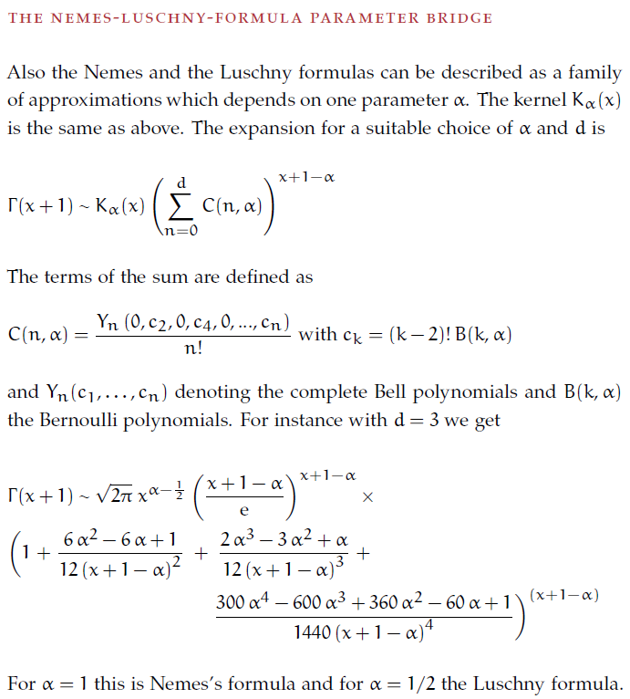
Maple
NemLusSer := proc(alpha,x,d) local kern, C, X;
X := x + 1 - alpha;
kern := sqrt(2*Pi)*x^(alpha-1/2)*(X/exp(1))^X:
C := n → CompleteBellB(n,0,seq((k-2)!*bernoulli(k,alpha),k=2..n)):
kern*add(C(n)/(n!*X^n),n=0..d)^X end:
# --- Test --- #
n:='n':alpha:='alpha':x:='x':d:=3:
NemLusSer(alpha,x,d); NemLusSer(1,x,6); NemLusSer(1/2,x,6);
evalf(subs(x=100,%%),32); evalf(subs(x=100,%%),32); evalf(factorial(100),32);
Miscellaneous notes
** The reference for the Ramanujan formula is: S. Raghavan and S. S. Rangachari (eds.) "S. Ramanujan: The lost notebook and other unpublished papers", Springer, 1988, p. 339. Ramanujan's statement is as follows:
Γ(x+1) = sqrt(Π)(x/e)^x (8x^3 + 4x^2 + x + θ(x)/30)^(1/6)
where θ(x) → 1
as x → ∞ and (3/10) < θ(x) < 1.
** Paul Abbott commented Ramanujan's statement on the Usenet (sci.math.num-analysis): "For
sqrt(Π)(n/e)^n*(n(4n(2n+1)+1)+(1/30)(1-(11/(8n))(1-(79/(154n))*
(1+(3539/(4740n))(1-(9511/(7078n))(1+90459/(152176n)))))))^(1/6)
one finds that
θ(x) = 1-11/(8x)+79/(112x^2)+3539/(6720x^3)-9511/(13440x^4)-30153/(71680x^5)
Clearly θ(x) → 1 for x → ∞. Also (3/10) < θ(x) < 1 for x >~ 1.3878. So this form does agree with Ramanujan's statement."
** Michael Hirschhorn [The Mathematical Gazette, Vol. 90, July 2006, 286-292] proved the following sharper bounds for Ramanujan's θ(x), valid for x > 6053/3987 (or x > 1.52).
1 - 11/(8x) + 5/(8x^2) < θ(x) < 1 - 11/(8x) + 11/(8x^2)
** The reference for Stieltjes' continued fraction formula is: M. Abramowitz, I. A. Stegun (eds.), Handbook of Mathematical Functions, p. 258, [6.1.48]. Note also: B. W. Char: "On Stieltjes' continued fraction for the gamma function", Mathematics of Computation 34, 150 (1980) 547-551.
** There are many Lanczos formulas for approximating n!. The form we use here is his equation (21) given in "A precision approximation of the gamma function", J. SIAM Numer. Anal., Ser. B, Vol. 1 (1964), pp. 86-96. Lanczos also devised other series (not included here) which might be more useful in practical computation. So he might not be fairly represented here! (Thanks to D. W. Cantrell for this remark.)
** The formulas of Warren D. Smith were taken from The Gamma function revisited, a typeset dated 29 Mar 2006.
** The formulas cantrell and wdsmith have an almost identical numerical performance.
** In our setup the approximation of Robert H. Windschitl is only a curiosity. Warren D. Smith's formula wdsmith*(n) provides a similar approximation based on Gamma(n+1/2). The two formulas wdsmith* and windschitl bracket the true value. (Note that our interpretation of the Windschitl formula differs from the interpretation used by W. D. Smith. However, our (Gamma-) interpretation seems to be more useful.)
| z | Windschitl | z! | W.D.Smith* |
| 0.0 | 0.999658 | 1.0 | 1.00429 |
| 0.5 | 0.88617 | 0.88623 | 0.88652 |
| 1.0 | 0.999984 | 1.0 | 1.000057 |
| 1.5 | 1.329333 | 1.329340 | 1.329361 |
| 2.0 | 1.9999954 | 2.0 | 2.0000107 |
**
I do not understand why the Windschitl formula is called 'a version suitable for calculators' on
Wikipedia and other web-sides. The appearance of sinh (or tanh in the case of
wdsmith*) make them look like stars of the 'Pimp My Formula' TV-show.
Well, it is time to un-pimp these formulas and to introduce the cute nemesGamma(n) and luschny*(n)
formulas, which are much simpler and computational less expensive but equal powerful. (For the
definitions see the paragraph Miscellaneous Approximations above.)
And there is an added value.
Comparing windschitl(n) with nemesGamma(n) we find the following approximation:
sqrt(x sinh(1/x)) = 1 + 1/(12 x^2 - 1/10) + O(x^(-6))
In fact | sqrt(x sinh(1/x)) - (1+1/(12 x^2-1/10)) | < 1 / (24192 x^6) .
Comparing wdsmith*(n) with luschny*(n) shows the approximation:
sqrt(x tanh(1/x)) = 1 - 1/(6 x^2 + 19/10) + O(x^(-6))
In fact | sqrt(x tanh(1/x)) - (1 - 1/(6 x^2 + 19/10)) | < 1 / (54 x^6) .
These two approximations are noteworthy. It does not make sense to replace the simple right hand sides by the functions on the left hand side in the above approximations to the factorial function as this will not decrease the approximation error. It will only produce pimped formulas ;-)
** Some numerical methods for computing x! (the tricks of the trade) can be found in the Handbook of Mathematical Functions (6.7).
** Let us define the Noerlund scheme as
noerlund(z,h,m)
ln(sqrt(2*Pi))+(z+h-1/2)*ln(z)-z+sum((-1)^(j+1)*bernoulli(j+1,h)/((j+1)*j*z^j),j=1..m-1)
The Noerlund scheme [Vorlesungen über Differenzenrechnung, Berlin 1924, p.111] gives us a common framework to classify approximation formulas to x!. There are three basic types, which correspond to our more general abbreviations kern#(x) used in the table above.
KERN0(x) = exp(noerlund(x+1,0,0)) = sqrt(2Pi/Y)*(Y/e)^Y where Y=x+1
KERN1(x) = exp(noerlund(x,1,0)) = sqrt(2Pi*Y)*(Y/e)^Y where Y=x
KERN2(x) = exp(noerlund(x+1/2,1/2,0)) = sqrt(2Pi)*(Y/e)^Y where Y=x+1/2
Note that KERN1 has a problem when x=0. Therefore KERN0 is to be preferred to KERN1. KERN2 has the most simple form and might be called the Hermite-Sonin variant.
** Asymptotic approximation of the Bernoulli Numbers.
Combining the nemes* formula and the well known connection of the Bernoulli Numbers with the Riemann Zeta Function we find the following remarkable formula, valid for even n >= 4.
|B(n)| ~ 2 sqrt(2 Pi n) ((n + 1/(12 n - 1/(10 n)))/(2 Pi e))^n
For example this approximation gives
| B(100) | ~ 0.28382249570691.. 10^79
compared with
| B(100) | = 0.28382249570693.. 10^79.
We can write this formula also as an approximation to Zeta(1-n), valid for even n >= 4.
| Zeta(1-n) | ~ 2 sqrt(2 Pi / n)((n / (2 Pi e))((120 n^2 + 9)/(120 n^2 - 1)))^n
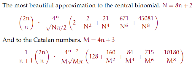
Asymptotic formulas for the central binomial coefficient
and the Catalan numbers.
The two asymptotic formulas for the central binomial coefficient and the Catalan numbers at the top of this page have a more precise (but less elegant) form which is:

More on this can be found in: Peter Luschny, "Divide, swing and conquer the factorial and the lcm{1,2,...,n}", preprint, April 2008. More coefficients, hints to the literature and to the interesting connection of coefficients with the Euler numbers can be found in the Online-Encyclopedia of Integer Sequences A220002 and A220422.

Asymptotic formulas for the Euler
and the Bernoulli numbers.
can be found here: Euler and Bernoulli.
Update-history.
=> Update September 23, 2016:
The most comprehensive study of approximations of the factorial (and Gamma function) to the present day is Weiping Wang, Unified approaches to the approximations of the gamma function, J. Number Theory (2016). However unfortunately Wang does not consider the efficient CF-approxi- mations discussed here.
=> Update June 13, 2013:
Lei Feng and Weiping Wang published six new formulas in their paper Two families of approximations for the gamma function. We added the most efficient one to the above data. It is a kern1 formula which performs under average. Feng and Wang cite parts of our tables but curiously they claim "these six formulae perform better than Nemes’ another result, which, to our knowledge, is numerically more accurate than all the other formulae presented in the literature ... as well as the other formulae in Luschny’s web page." Apparently they totally misunderstood the structure of our tables and how we have set up the successive approximations of a formula.
=> Update Nov 30, 2012:
Prof. Neven Elezović kindly pointed out an error in the asymptotic formula of the Catalan numbers on the top of this page: 10177 has to be replaced by 10180. Now corrected. Thanks!
=> Update Jun 3, 2011: A formula of T. Buric and N. Elezović added.
Formula (3.3) in "New asymptotic expansions of the gamma function and improvements of Stirling’s type formulas."
1000!           0.402387260077093773543702433923003*10^2568
Buric-Elezović: 0.402387260077093773543702433922664*10^2568
StirlingSeries: 0.402387260077093773543702433922668*10^2568
There is no noticeable difference (in terms of significant decimal digits) compared to the Stirling series. The Stirling series (see the formulas for stirser above) has smaller coefficients and is simpler.
=> Update Mar 24, 2011: More annoying things from Cristinel Mortici!
Cristinel Mortici writes in: "A substantially improvement of the Stirling formula", to appear in: Applied Mathematics Letters.Received date: 30 August 2009.
"We introduce the new approximation formula
n! ~ sqrt(2 π n)(n/e + 1/(12 e n))^n = μn (1.1)
which has great superiority over all the previous formulas. ... but our new formula (1.1) has the advantage of simplicity. ... Unlike most formulas which are variations of the asymptotic expansion of the Stirling formula, our formula (1.1) has an original construction mode. ... Our new approximation formula n! ~ μn gives surprisingly good results. It is much better than the Gosper's approximation n! ~ γn. "
Fact is: Formula 1.1 is on this page since Nov 12, 2006. "The new approximation formula" and its "original construction mode" are due to Gergő Nemes. It is described here as the nemes1 formula. But much more is true: Nemes went ahead and gave a full expansion to an asymptotic approximation of the factorial function. And Nemes published his results also in other places: First version, second version, third version.
=> Update Feb 5, 2011: New approximation added. And read about Cristinel Mortici!
Gergő Nemes has published a clever and efficient new formula! [Nemes] I include the formula under the name NemesG in the tables above. The new formula scores 12 (!) times as the best result in the tables! Well done, Gergö. This was the good news.
Now some other news. The Comptes Rendus de l'Académie des Sciences, Paris, Ser. I 348 (2010) 137–140, presented by Jean-Pierre Kahanep, begins: "The purpose of this Note is to construct a new type of Stirling series, which extends the Gosper’s formula for big factorials." It ends: "Finally, we demonstrate the superiority of our new series..."
OK, so I had to include it here, n'est-ce pas? Well, not really. It is already here, for many years. It is the Wehmeier formula. So perhaps there is a new idea in deriving this formula? The author, Mortici, says the basic tool is a lemma which "..was used by Mortici.." several times. Looking at the lemma I see that it is exactly the way Wehmeier derived his formula. So Mortici's result is neither 'new' nor does the above table indicate any 'superiority' of the formula. On the other hand Wehmeier never published his result (Mortici publishes every month or so a 'new sharp' approximation to the 'big factorials'). Wehmeier just participated in a discussion on the Usenet group de.sci.mathematik. It is nice to know that once upon a time, before the cranks took over, a discussion on dsm could be on the level of the Comptes Rendus de l'Académie des Sciences, Paris. [Mortici] [dsm1] [dsm2]
=> A000207 at OEIS.
Recently (Feb 2007) Rainer Rosenthal drew my attention to the number of planar 2-trees, sequence A000207 at OEIS. The sequence can be computed as (Maple):
A000108 := n -> (2*n)! / (n!*(n+1)!);
A000207 := n -> A000108(n)/(2*n+4)+ A000108(floor(n/2))* (3-modp(n,2))/4 +
               `if`(modp(n,3)=1,A000108(floor((n-1)/3))/3,0);
I noticed that the quotient A000207(n+1) / A000207(n) has a remarkable regular asymptotic expansion:
QuotAsymptotic := n -> 4 - (10/n)* (1-(3/n)* ((1-(3/n)* ((1-(3/n)* ((1-(3/n)
                       *((1-(3/n)*((1-(3/n)*((1-(3/n)))))))))))))).
=> Update Jan 11, 2007: The computation of Stieltjes' continued fraction.
After calculating his famous continued fraction for the Gamma function Stieltjes remarked: "Le calcul est trés pénible ... la loi de ces nombres paraît extrêmement compliqué". I looked at the state of the art and wrote a summary. See the link list below.
=> Update Jan 9, 2007: Two new continued fraction approximations added.
My latest additions are the formulas luschnyCT and nemesCT. A first comparison shows that the luschnyCT formula performs slightly better than Stieltjes' formula (or the W.D.Smith or Cantrell formula).
=> Update Jan 4, 2007: Three simple but powerful formulas added.
The formulas nemes*, nemesGamma and luschny* are new. They are much simpler than the windschitl or wdsmith* formulas but equal powerful.
=> Update Dec 28, 2006: The Luschny formulas added.
The new Luschny formulas added following Sonin's 'half-shift' idea and similar to the Nemes approach.
=> Update Dec 14, 2006: The Gosper-Smith formulas added.
Gosper's z! ~ sqrt((2*z+1/3)*Pi)*(z/e)^z recasted by W. D. Smith following Sonin's 'half-shift' idea.
=> Update Dec 13, 2006: Warren D. Smith's formulas added.
The continued fraction formulas of W. D. Smith are based on the Hermite-Sonin discussion: Sur les polynômes d'Bernoulli, Extrait d'une corres-pondance entre M. Sonin et M. Hermite. J. für Math. 116 (1896), 133-156.
=> Update Nov 18, 2006: The Continued Fraction Formula corrected
Gergő Nemes spotted an error in stieltjes3. Thanks, Gergő! With this correction, the author hopes that the formulas are now error-free.
=> Update Nov 12, 2006: The Nemes Formula announced
Gergő Nemes, a student from Hungary, sent me his formula. Thank you Gergő for sharing your findings with us!
 |
=> Update Nov 9, 2006: The Wehmeier Formula rediscovered
 |
In expanded normal form:
 |
First I thought that I had discovered a new family of formulas. However, a closer examination showed that I had rediscovered the Wehmeier formula while I was contemplating the Ramanujan formula. Nevertheless, I left the L-formula in the table because I think this alternative way to look at the Wehmeier formula throws some light on the structure of the Ramanujan formula.
=> Update Aug, 2006: S. Ramanujan's Formula
 |
In expanded normal form:
 |
Formulas on the OEIS
|
|
Links
OEIS A119422
* Knud Thomsen's formula for small positive values
* Stefan Wehmeier's announcement of his approximation.
* G. R. Pugh's thesis "An analysis of the Lanczos gamma approximation"
* Hugo Pfoertner's Fortran implementation of Cantrell's expansion.
* 'Calculators and the Gamma Function' about the origin of the Windschitl-formula.
* The computation of Stieltjes' continued fraction.
(C) Peter Luschny, 2004-2016. Free under the Creative Commons Attribution-ShareAlike 3.0 Unported License (the same license which Wikipedia uses). You can download this page as a pdf-file.
Cite this as: Peter Luschny, "Approximation Formulas for the Factorial Function".
Web. Accessed September 23, 2016. Available http://www.luschny.de/math/factorial/approx/SimpleCases.html.
Save your integrity and cite this page if you have used it or even copied from it! Do not claim that something is new if it has been on this page for many years and discussed in public places. 'Copy and paste' is no peccadillo! If you work as a referee do not force others to cite your work even if it is unrelated. These remarks clearly also apply to Cristinel Mortici.
![]() Back to the Homepage of Factorial Algorithms.
Back to the Homepage of Factorial Algorithms.