GFUN
A Sage Toolbox for the OEIS
Part 1: Basic operations
A generating function is a formal power series \(a(x) = \sum_{n=0}^\infty a_n x^n\) which lets us calculate with the sequence \((a_0,a_1,a_2,...)\) as if it were an analytic function. Compared with the ring of sequences the ring of power series has two great advantages: It is an integral domain (which the ring of sequences is not) and its multiplication, the Cauchy product, has a natural combinatorial interpretation.
Gfun is a classic Maple package for the manipulation of generating functions by Bruno Salvy and Paul Zimmermann written in 1994 (Gfun, swmath). We borrow the name gfun and intend to provide in a series of posts on this blog a similar toolbox, implemented in Sage and geared for the use with the OEIS. In this post we start with the most basic operations and examples.
Our implementation is object oriented and is hopefully easier and more intuitive. We illustrate this with an example, the computation of A048172.
The Maple version:
with(gfun):
f := series((ln(1+x)-x^2/(1+x)), x, 21):
egf := seriestoseries(f, 'revogf'):
seriestolist(egf, 'Laplace');
The same with our Sage toolbox:
gf = log(1+x)-x^2/(1+x)
gfun(gf, 'rev').as_egf()
The constructor gfun (g, op) has two arguments, g a symbolic expression in one or two variables and op the name of an operation according to the table below. It returns an object representing a formal power series which can be accessed through the methods listed below.
The operations op:
- None ... g unmodified (the default without parameter).
- 'rev' ... compositional inverse of g.
- 'inv' ... multiplicative inverse of g.
- 'exp' ... exponential of g.
- 'log' ... logarithm of g.
- 'int' ... formal integral of g.
- 'der' ... formal derivative of g.
- 'logder' .. logarithmic derivative of g.
The methods
The methods return the sequence of coefficients of the represented power series up to the given precision prec (which is by default 12). The type of the power series is indicated by the method name. The types are 'ogf' (ordinary power series), 'egf' (exponential power series), 'lgf' (logarithmic power series) and 'bgf' (binary power series).
- as_ogf (prec=12, search=false)
- as_egf (prec=12, search=false)
- as_lgf (prec=12, search=false)
- as_bgf (prec=12, search=false)
- as_series (prec=12, typ='ogf')
Setting the parameter 'search=true' (default is false) will look up related information in the OEIS provided you are connected with the Internet.
In the bivariate case (i. e. the given symbolic expression depends on two variables x and t) 'coeffs' returns a triangular table giving the coefficients of those polynomials which are the coefficients of the power series when expanded in t. 'values' returns a rectangular array displaying the values of these polynomials evaluated at the nonnegative integers. The values method evaluates the n-th polynomial in the n-th column of the rectangular array. The 'colgenerator' returns a rational generating function of the n-th column of the values array.
- coeffs (typ='ogf', rows = 8)
- values (typ='ogf', rows = 8, cols = 8)
- pred (typ='ogf', rows = 8)
- succ (typ='ogf', rows = 8)
- colgenerator (n, typ='ogf')
The methods 'pred' (short for predecessor) and 'succ' (short for successor) are two transformations which map integer triangles to integer triangles. 'succ' lists the numerators of the partial fraction decomposition of the generating functions of the columns of the value array as an triangular array. And 'pred' is the transformation inverse to 'succ'. Many examples show that these transformations lead to interesting and meaningful new integer triangles.
Example use
The toolbox gfun.sage can be downloaded from github. To load the toolbox we have to execute the next command first. The path must of course be adapted to the computing environment.
attach('~/.sage/gfun.sage')
x = SR.var('x')
cato = (1-2*x-sqrt(1-4*x))/(2*x)
Note: The type of input gfun expects is a symbolic expression. ('SR' in 'x = SR.var('x')' stands for Symbolic Ring.)
gf = gfun((1-2*x-sqrt(1-4*x))/(2*x))
print gf.as_ogf()
print gf.as_ogf(6)
If you want more (or fewer) terms of the sequence call as_ogf with this value. You can also call as_ogf without a value. Then the default length (= 12) is used.
You don't have to re-execute gfun to get a different length of the sequence. The returned object behaves as if it can provide unlimited access to the sequence. This is in contrast to the way some similar (Maple, Mathematica) libraries work which can be found in the OEIS. These programs work on lists; there you have to assign a fixed length at the start which you can't change afterwards. More generally the objects in these libraries behave like 1-based lists whereas the objects here behave like 0-based sequences.
You also can execute different 'as_xgf' methods on the same object. In combination with the operations this gives a multitude of different representations of sequences.
The bivariate case.
The Motzkin polynomials, A097610.
x, t = SR.var('x, t')
motzkin = gfun((1-t*x-sqrt((x^2-4)*t^2-2*t*x+1))/(2*t^2))
motzkin.as_ogf(5)
motzkin.coeffs()
Motzkin polynomials evaluated at the integers, A247495.
motzkin.values()
Using the rational generating functions of the columns gives the array with rows and columns exchanged.
for n in range(8):
gf = motzkin.colgenerators(n)
print gfun(gf).as_ogf(7)
The column generating functions are given in the form of partial fractions.
for n in range(6):
print motzkin.colgenerators(n)
Collecting the numerators of these partial fractions gives (apart from the signs) the number triangle A247497 which we call the 'associated Motzkin numbers'. This triangle with column k divided by k! is the successor triangle of the Motzkin triangle, motzkin.succ[n,k] = A247497(n,k)/k!.
motzkin.succ()
The first column lists the Motzkin numbers and the second column A058987 Catalan(n) - Motzkin(n-1). The next to last column are the triangular numbers A000217.
Summary: We started with the Motzkin polynomials A097610, looked at the Motzkin values A247495 and arrived via the partial fractions of the column generating functions at the associated Motzkin numbers A247497 which include the Motzkin numbers A001006 as a special case.
The exact definitions of the 'pred' and 'succ' transformations and many more examples are given in this blog post.
- explore_values(g, typ='ogf', rows=6, cols=6)
This methods is a convenience function. Given a bivariate generating function g it searches the OEIS for information about sequences in the rows and columns of the value table (you have to be online). It helps to quickly get an overview of the situation and to build a cross-reference table like the one given above.
For instance the call
gfun.explore_values(motzkin)
tries to find information about the first 6 rows and the first 6 columns of the array of Motzkin values.
- explore_genfun(g)
Given an univariate generating function g this method searches for all combinations of the above operations with the above methods which make mathematical sense and give an integer sequence. If such sequences exist it will search the OEIS for information about these sequences.
The information provided by explore_genfun() is often very useful while studying a sequence, sometimes even more useful and inspiring than the information returned by the SuperSeeker. This is because it does not only hint to information that can be found in the OEIS but also indicates what possible valuable information is missing. Note that you have to be connected to the internet to use this method and it may take some time to finish. (See the example at the end of this post.)
After the method has finished it displays a plot which is a kind of a fingerprint of the generating function. A green path indicates that there are related sequences in the OEIS (which are listed in the output), a red path indicates that in this case a meaningful integer sequence exists which is apparently not in the database. In the other cases for one reason or another there is no related integer sequence.
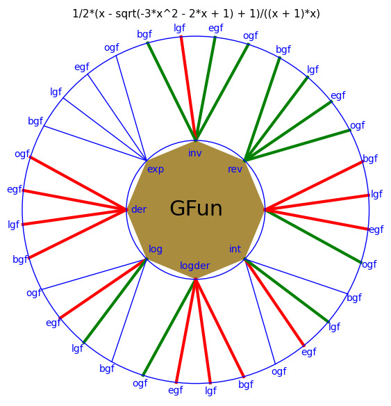
This plot is a snapshot of the current situation for the Riordan numbers. It was generated by the commands:
x = SR.var('x')
riordan = (1+x-sqrt(1-2*x-3*x^2))/(2*x*(1+x))
gfun.explore_genfun(riordan)
All sequences here are by definition functions from N = {0,1,2,3,...} to some codomain. Triangles and rectangles are functions from N X N to some codomain. In other words all sequences have 'offset' 0 and all two-dimensional arrays are (0, 0) based. Lists in the OEIS might deviate from this: often they have (1, 1) or (1,0) or (0,1) as base-point of enumeration. This means that references to the sequences in the OEIS are always modulo the different conventions.
-
GFUN — A Sage Toolbox for the OEIS
Part 1: Basic operations- Introduction
- Examples for generating functions
- Riordan numbers
- Lucas numbers
- Squares of Pell numbers
- Balanced parentheses of two types
- The derivative of Cato
- Generalized Fibonacci numbers
- Generalized Catalan numbers
- Little Narayana polynomials
- Large Narayana polynomials
- Further remarks on Narayana polynomials
- Scaled Legendre polynomials
- Lah polynomials
- Eulerian polynomials
- The harmonic polynomials
- Further remarks on harmonic polynomials
- Generalized Lucas Numbers
- Some Riordan arrays
- Series inversion, the multiplicative inverse.
- Partition numbers
- Euler numbers
- Swiss-Knife Polynomials
- Reversion, the compositional inverse.
- Large Schröder numbers
- Generalized Motzkin numbers
- Searching the OEIS
- Exploring the generating function
What you are reading is in fact an HTML-rendered IPython notebook which explains the use of the toolbox by examples.
Riordan numbers
A005043, OGF
x = SR.var('x')
riordan = gfun(2/(1+x+sqrt((1+x)*(1-3*x))))
riordan.as_ogf()
Or written in one line:
gfun(2/(1+x+sqrt((1+x)*(1-3*x)))).as_ogf()
A005043, EGF
x = SR.var('x')
riordanE = gfun(exp(x)*(bessel_I(0, 2*x)-bessel_I(1, 2*x)))
riordanE.as_egf()
Or written in one line:
gfun(exp(x)*(bessel_I(0, 2*x)-bessel_I(1, 2*x))).as_egf()
lucas = gfun(-log(1/(x^2 - x - 1)))
lucas.as_lgf()
Squares of Pell numbers
A079291, LGF
pellsqr = gfun(log((1+2*x+x^2)/(1-6*x+x^2))/8)
pellsqr.as_lgf(10)
Balanced parentheses of two types
A151374, BGF
catalan = gfun((1 - sqrt(1 - 4*x))/(2*x))
catalan.as_bgf()
The derivative of Cato
Cato is a nickname for Cata-lan with first term 0. A245391, BGF
cato = (1 - sqrt(1 - 4*x) - 2*x)/(2*x)
print gfun(cato, 'der').as_bgf()
gfun(1/(1 - x - x^2)).as_ogf()
This is case n=2 of the generalized Fibonacci numbers.
genFibo = lambda n: (1-sum(x^j for j in (1..n)))^(-1)
for n in range(0,9):
print gfun(genFibo(n)).as_ogf()
gfun((1-x)/(1-2*x)).as_ogf()
x, t = SR.var('x, t')
genCatalan = gfun((1-t*x-sqrt(x^2*t^2-2*t*x-4*t+1))/(2*t))
genCatalan.coeffs()
genCatalan.values()
This table can be found in A247507 showing how many sequences in the OEIS are related to this generating function.
genCatalan.succ()
genCatalan.pred()
x, t = SR.var('x, t')
littleNarayana = gfun((t*(1-x)-sqrt((t*(x-1))^2-2*t*(x+1)+1))/(2*t))
print littleNarayana.as_ogf(5)
littleNarayana.coeffs()
littleNarayana.values()
The same table, with rows and columns interchanged, can be found in A243631, showing how many sequences in the OEIS are related to this generating function.
littleNarayana.succ()
littleNarayana.pred()
x, t = SR.var('x, t')
largeNarayana = gfun((t*(x-1)-sqrt((t*(x-1))^2-2*t*(x+1)+1))/(2*t*x))
print largeNarayana.as_ogf(5)
largeNarayana.coeffs()
largeNarayana.values()
largeNarayana.succ()
largeNarayana.pred()
For the reason of reference we add explicit definitions of the two kinds of Narayana polynomials. Note that both kinds give the Catalan numbers in row 1 in the tables above. The brand-mark is row 2: the little Narayana polynomials give the little Schröder numbers and the large Narayana polynomials the large Schröder numbers.
# Little Narayana polynomials:
def liN(n, x):
    N = lambda n,k: binomial(n,k)^2*(n-k)/(n*(k+1))
    return expand(add(N(n, k)*x^k for k in range(n))
           if n>0 else 1)
# Large Narayana polynomials:
def laN(n, x):
    N = lambda n,k: binomial(n+1,k)*binomial(2*n-k,n)/(n+1)
    return expand(add(N(n,k)*(x-1)^k for k in range(n+1)))
Scaled Legendre polynomials
2^n*P_n(x), A157077, bivariate BGF
legendre = gfun((1-2*x*t+t^2)^(-1/2))
print legendre.as_bgf(5)
legendre.coeffs('bgf')
legendre.values('bgf')
legendre.succ('bgf')
legendre.pred('bgf')
Lah polynomials
A111596, bivariate EGF
x, t = SR.var('x, t')
lah = gfun(exp(x*t/(1-t)))
lah.as_egf(7)
lah.coeffs('egf')
lah.values('egf')
lah.succ('egf')
lah.pred('egf')
Eulerian polynomials
A173018, bivariate EGF
x, t = SR.var('x, t')
eulerian = gfun((x-1)/(x-exp(t*(x-1))))
print eulerian.as_egf(5)
eulerian.coeffs('egf')
eulerian.values('egf')
eulerian.succ('egf')
eulerian.pred('egf')
The harmonic polynomials
A109822, bivariate EGF
x, t = SR.var('x, t')
harmonic = gfun(1 + x/(1-x)*(1/(1-x*t)^(1/x)-1/(1-x*t)))
print harmonic.as_egf(5)
harmonic.coeffs('egf')
harmonic.values('egf')
harmonic.succ('egf')
harmonic.pred('egf')
Why call these polynomials 'harmonic polynomials'? Because they evaluate at x=1 to the harmonic numbers H(n) like this: H(n) = harmonic(n, 1) / n!.
P = harmonic.as_egf()
print [p(x=1)/factorial(n) for (n, p) in enumerate(P)]
The generating function of the harmonic numbers:
H = gfun(1-log(1-x)/(1-x))
print H.as_ogf()
Note that these polynomials also give nice values at x = -1, the order of alternating group A_n, A001710.
print [(-1)^n*p(x=-1) for (n, p) in enumerate(P)]
Generalized Lucas Numbers
A247505, parametrized LGF
x = SR.var('x')
genLucas = lambda n: -log((1+sum((-1)^(j+1)*x^j for j in (1..n)))^(-1))
for n in (0..9):
print gfun(genLucas(n)).as_lgf()
Note that the limiting case n → oo is A000225 and that the main diagonal is also this sequence. This is another case of compositional convergence.
A000225 = exp(2*x) - exp(x)
gfun(A000225).as_egf()
x, t = SR.var('x, t')
rarr = lambda n: -log((1/x+sum((-1)^(j+1)*t^j for j in (1..n)))^(-1))
gfun(rarr(2)/x).coeffs('lgf')
rarr(3) / x = (log(t^3-t^2+t+1/x))/x
gfun(rarr(3)/x).coeffs('lgf')
Now, to what limit does the sequence of these triangles (in their non-truncated form) converge to for n → oo? It's A206735, a variant of Pascal's triangle!
x, t = SR.var('x, t')
A206735 = gfun((1-2*t+(1+x)*t^2)/(1-2*t+(1+x)*t^2-t*x))
print A206735.as_ogf(5)
A206735.coeffs('ogf')
The call gfun(g, 'inv') returns an object which represents the multiplicative inverse of g. That is, seen as a formal power series, g multiplied with the inverse of g is the formal power series equivalent to 1. g has an inverse in this sense if and only if g(0) ≠ 0. In the case g(0) = 0 you will get the error message "ValueError: Series must have valuation zero for inversion."
Partition numbers
A000041, inverse OGF
g = lambda n: mul((1 - x^k) for k in (1..n))
n = 20
print gfun(g(n), 'inv').as_ogf(n)
x = SR.var('x')
euler = cosh(x)
s = gfun(euler, 'inv')
print s.as_egf()
x = SR.var('x')
gf = exp(-x)*cosh(x)
s = gfun(gf, 'inv')
print s.as_egf()
Swiss-Knife Polynomials
A153641, bivariate EGF
x, t = SR.var('x, t')
sk_poly = gfun(exp(x*t)*sech(t))
print sk_poly.as_egf(5)
sk_poly.coeffs('egf')
sk_poly.values('egf')
Note that the first two rows are the two flavors of the Euler numbers. Thus the Swiss-Knife polynomials can be seen as a generalization of the Euler numbers.
sk_poly.succ('egf')
sk_poly.pred('egf')
Reversion, the compositional inverse.
The call gfun(g, 'rev') returns an object which represents the compositional inverse of g.
- For reversion g (as a series) must have valuation one (the coefficient g(0) must be 0). The returned series is then the compositional inverse of g (with respect to the formal power series u with one nonzero coefficient, u(1) = 1).
- If g is not invertible in the sense above (i. e. if g(0) != 0) then the reversion will be computed as follows:
    r = g / g[0]
    r = r.shift(1)
    r = r.reversion()
    r = r.shift(-1)
    r = r * g[0]
If you wish to turn off this extension you can call
g.strict_reversion(true)
and revert this by setting g.strict_reversion(false).
If strict reversion is in effect you will get instead the error message "ValueError: Series must have valuation one for reversion."
Note that the default behavior is the extended form as this is in the context of the OEIS more useful in many situations.
Large Schröder numbers
A006318, reversion OGF
x = SR.var('x')
schroeder_L = gfun((1 - x)/(1 + x), 'rev')
schroeder_L.as_ogf(9)
x = SR.var('x')
genMotzkin = lambda n: 1/(1+sum(x^k for k in (1..n)))
for n in range(9):
print gfun(genMotzkin(n), 'rev').as_ogf()
Limiting case n → oo Catalan numbers, A000108. Also note that the main diagonal are the Catalan numbers.
catalan = gfun((1-sqrt(1 - 4*x))/(2*x))
catalan.as_ogf()
Let's come back to our first example.
x = SR.var('x')
riordan = gfun(2/(1+x+sqrt((1+x)*(1-3*x))))
riordan.as_ogf()
If you call as_ogf() with the additional parameter 'search=true' you get:
riordan.as_ogf(search=true)
You will receive up to four proposals for related sequences from the OEIS (including the first terms so that you can immediately check the similarity of the terms). The prerequisite is that the computer is connected to the Internet. Of course the same works for the functions as_egf(), as_lgf() and as_bgf().
Putting everything together we get the method gfun.explore(). The output has the format:
'op' as_xgf [0, 1, 2, ...]
A000000 (1, 1, 2, ...)
A111111 (1, 1, 1, ...)
A222222 (1, -1, -1, ...)
.....
'op' will be one of the eight operations
[None, 'rev','inv','exp','log','der','logder','int']
and 'as_xgf' one the four representations
['as_ogf', 'as_egf', 'as_lgf', 'as_bgf'].
All 32 combinations will be tested and those giving meaningful results will be reported. You have to be online to get results and it takes a while. The function will print 'Done!' when finished.
After the method has finished it displays a plot which is a kind of fingerprint of the generating function. A green path indicates that there are related sequences in the OEIS (which are listed in the output), a red path indicates that in this case a meaningful integer sequence exists which is apparently not in the database. In the other cases for one reason or another there is no related integer sequence.
x = SR.var('x')
riordan = (1+x-sqrt(1-2*x-3*x^2))/(2*x*(1+x))
gfun.explore(riordan)