Here is an alternative version which requires mathematical fonts and JavaScript enabled. It is rendered by MathJax [see here] and better readable.
Is the Gamma function mis-defined?
Or: Hadamard versus Euler -
Who found the better Gamma function?
[A picturesque account.]
Abstract. The Gamma function of Euler often is thought as the only function which interpolates the factorial numbers n! = 1,2,6,24,.... This is far from being true. We will discuss four factorial functions
- the Euler factorial function n!,
- the Hadamard Gamma function H(n),
- the logarithmic single inflected factorial function L(n),
- the logarithmic single inflected hyper-factorial function L*(n).
We will show that these alternative factorial functions posses qualities which are missing from the the conventional factorial function but might be desirable in some context.
The problem of interpolating the values of the factorial function n! = 1,2,6,24,... was first solved by Daniel Bernoulli and later studied by Leonhard Euler in the year 1792 (see [history]). The interpolating function is commonly known as the Gamma function.
However, this function has an unpleasant property: If n = 0,-1,-2,... then Gamma(n) becomes infinite.
Fig. 1: Bernoulli's Gamma function, interpolating n!, n integer.
What is not so well known is the fact, that there are other functions which also solve the interpolation problem for n! and behave much nicer. A particular nice one was given by Jacques Hadamard in 1894.
Hadamard's Gamma-function has no infinite values and is provable simpler then Euler's Gamma-function in the sense of analytic function theory: it is an entire function.
The following figures give a first idea what the Hadamard Gamma-function looks like.
Fig. 2: Hadamard's Gamma function, interpolating n!, n integer.
Formulas for the Hadamard Gamma Function H(x)
Hadamard's Gamma function is defined as
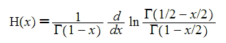
If we introduce the Digamma (Psi) function
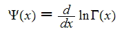
we can write in equivalent form

There is a second approach which shows the intuitive meaning of Hadamard’s function more clearly. Let us define the function Q(x) by the next expression:

The graphs of Q(x) [red] and of 1 - Q(x) [green] are shown in the next plot:
Fig. 3: Q(x) [red], the 'oscillating factor' in Hadamard's Gamma function.
The graph of Q(x) looks like an approximation to the indicator function of the positive real numbers. Now let us consider the product of this function and Gamma(x). Then we have the following identity for Hadamard's Gamma function:
H(x) = Gamma(x) Q(x-1/2)
For x=0,-1,-2,-3,... H(x) is defined by the value of the limit.
A New Factorial Function L(x)
There is another factorial function, proposed by Peter Luschny in October 2006, which is also continuous at all real numbers and which we will compare to Hadamard's Gamma function.

Fig. 4: Luschny's factorial function L(x).
Interpolating n!, n integer > 0. [L(0)=1/2]
The following figure compares the Luschny factorial L(x) with the Euler factorial (x! = Gamma(x+1)) for nonnegative real values.
Fig. 5: Factorial x! [red] and the L-factorial L(x) [green]
Crucial for the definition of the L-factorial are the functions
| g(x) = (x/2) (Psi(x/2 + 1/2) - Psi(x/2)) - 1/2 [*] |
| P(x) = 1 - g(x) sin(Pi x) / (Pi x). [**] |
We set P(0) = lim [x->0] P(x) = 1/2. The graph of P(x) is shown in the next plot:
Fig. 6: The 'oscillating factor' of the L-factorial.
P(x) [red] and 1 - P(x) [green].
The definition of the L-factorial [7] is
| L(x) = x! P(x). |
For x=0,-1,-2,-3,... L(x) is defined by the value of the limit. Note that L(-x) = (-x)! (1 - P(x)).
Luschny's factorial function L(x) approximates the non integral values x > 0 of the factorial function better then Hadamard's Gamma function H(x) the non integral values x > 0 of the Gamma function. Compare figure 7.
Fig. 7: Gamma(x) - H(x) [red] and x! - L(x) [green]
A Family of Approximate Gamma functions.
To understand the relation between Hadamard's Gamma function and Luschny's factorial
function better we consider a common generalization. To this end we introduce
| g(x, alpha) = (x/2) (Psi(x/2 + 1/2) - Psi(x/2)) - alpha/2, |
| P(x, alpha) = 1 - g(x, alpha) sin(Pi x) / (Pi x), |
| L(x, alpha) = x! P(x, alpha). |
Obviously L(x) = L(x, 1) and it is easy to see from the functional equation of Psi that H(x+1) = L(x, 2).
... and now for values x < 0 .
Starting from the idea of interpolating n! = 1,2,6,24,... one expects a factorial function for arbitrary real numbers x to be monotonically increasing for all x. It comes almost as a shock to see that the Euler factorial behaves very differently from this expectation for real numbers x < 0. On the other hand, the behavior of the L-factorial meets our expectations. The following plot compares the logarithm of both functions:

Fig. 8: log(abs((x+1)!)) [green:x<0, red:x>0] and log(L(x+1)) [red]
Convexity and the Bohr-Mollerup-Artin theorem.
Hadamard looked at his formula from the point of view of analytic function theory, as is emphasized by the title of his paper "Sur L'Expression Du Produit 1.2.3...(n-1)... Par Une Fonction Entière" [2]. However, at the turn of the century (1900) new ideas came up and influenced the way the Gamma function was looked at. Philip J. Davis writes in his exposition [1, p.867] :
"Aesthetic conditions were not to be found in the older, analytic considerations, but in a newer, inner, organic approach to function theory which was developing at the turn of the century. Backed up by Cantor's set theory and an emerging theory of topology, the new function theory looked not so much at equations and identities as at the fundamental geometrical properties. The desired condition was found in notions of convexity."
Only many years after Hadamard defined his Gamma function this more geometric view of the Gamma function was fully understood. It cumulated 1922 in a characterization of the Gamma function by logarithmic convexity which is now known as the Bohr-Mollerup-Artin theorem.
The Dints in Hadamard's Gamma function.
Let us now examine Hadamard's Gamma function from the geometric point of view.
Fig. 9: (log(H(x))'' [red] and (log(L(x))'' [green]
Figure 9 shows the behavior of H(x) and L(x) with regard to logarithmic convexity. Whereas the logarithm of the L-factorial has only one inflection point (this is the point where (log(L(x))'' changes the sign near x=1), Hadamard's Gamma function has many inflection point: H(x) is not logarithmic convex for x > 1. The regions where (log(H(x))'' < 0 and x > 1 might be visualized as small dints in Hadamard's function. And the presence of these dints might be regarded as a flaw in Hadamard's definition.
Moreover, in contrast to the H-Gamma function the L-factorial is not only free from dints but approximates the logarithmic behavior of the Euler Gamma function with positive values as x goes to +/-infinity. The next figure shows (log(L(x))'' in comparison to (log(Gamma(x))'' (for x>0) and -(log(Gamma(-x))'' (for x<0).
Fig. 10: (log(L(x))'' [red] and sign(x)(log(Gamma(sign(x)x))'' [green]
Single Inflected Logarithmic Convexity.
To conceptualize our findings we introduce the following definition.
DEFINITION: A function is lsi-convex if and only if it is defined for all real x and is logarithmic convex for x > C for some C and logarithmic concave for x < C. ('lsi' is an acronym for 'logarithmic single inflected'.)
As our discussion showed, the H-Gamma function is not lsi-convex, but the L-factorial is lsi-convex. This is not difficult to prove if we look at V(x) = (log(L(x))'' and observe that if c = 1.073536774.. and x > c then V(x) > 0 and V(x) < 0 for x < c. In fact V(x) > 1/(x+2) for x > 2, V(x) < -1/x^2 for x < -3 and the only zero of V in the interval [-3, 2] is c. (Compare figure 11.)
Fig. 11 V(x) = (log(L(x))'' [red] and bounds [green]
If we choose alpha = 1.031474316... in the generalized formula L(x, alpha) the inflection point (point of change in concavity) is exactly 1.
A Wish List
The Euler factorial x! = Gamma(x + 1) is a function
[1] which is positive for x > 0,
[2] is 1 at x = 1,
[3] is logarithmically convex for x > 0,
[4] and interpolates n! (n>0 integer).
However, contemplating Figure 8 we might also ask for a function
[1*] which is positive for all real x,
[2*] is 1 at x = 1,
[3*] is logarithmically convex if x>c and logarithmically concave if x<c (for
some c),
[4*] and interpolates n! (n>0 integer).
Note that the postulates [n*] are a superset of the postulates [n]. The L-factorial satisfies the postulates [n*], but the H-Gamma function does not.
The Approximate Functional Equation and an Error Estimate
Now what about the functional equation F(x+1)/((x+1)F(x)) = 1 for x > 0? This
identity holds for the Euler factorial exactly but for the H-Gamma function and
the L-factorial function only approximately. Figure 12 displays how wide they are
off the unit.
Fig. 12: The approximate functional equation.
(x+1)!/((x+1)x!) [black], L(x+1)/((x+1)L(x)) [red], H(x+1)/(xH(x)) [green].
In the case of the L-factorial this approximate functional equation is approximated by the function (x =/= 0)

It is clear that L(x) is asymptotical equal to x!. The formula for the approximate functional equation might be translated into the error bound L(x) / x! < 1 + 1/(2Pi x) (if x>1).
Fig. 13: L(x)/x! [green] and the bound 1+1/(2Pi x) [red].
The Functional Equation of L(x, alpha)
Of course our factorial functions obey also a full functional equation, not only an approximate one. And the L-factorial does have a simple functional equation. This can be easily seen from the definition. We find
L(1+x) - (1+x)L(x) = (1/2) x! sin(PIx)/(PIx) = (1/2) / (-x)! .
Thus the functional equation of the L-factorial is
| L(1+x) = (1+x)L(x) + (1/2) / (-x)! . |
The general case is
| L(1+x, alpha) - (1+x)L(x, alpha) = |
| = ((1-alpha)x + 1 - alpha/2) x! sin(PI x)/(PI x) |
| = ((1-alpha)x + 1 - alpha/2)/(-x)! |
and gives the general functional equation
L(1+x, alpha) = (1+x)L(x, alpha) + ((1-alpha)x + 1 - alpha/2) / (-x)! .
From the results and methods of [3] we conclude that each meromorphic solution of this functional equation is a transcendental differential function over the differential field of complex rational functions.
The function g(z) and the product z!(-z)!.
We prove the following identity
| g(z) + g(-z) = z! * (-z)! |
Proof:


In the last step we used the well known identity (Ergänzungssatz, L. Euler,
1749) 
Another application of Euler's reflection equation is the identity
| L(-z) = g(z) / z! |
Proof:
L(-z) = (-z)! P(-z) = (-z)! (1 - P(z))
= (-z)! g(z) sin(Pi z) / (Pi z)
= (-z)! g(z) / ((-z)! z!) = g(z) / z!
The reflection products z!(-z)! and L(z)L(-z).
Let us compare the reflection equation of the Euler factorial with the reflection equation of the L-factorial. To this end we introduce the function
Lambda(z) = L(z) L(-z)

Fig. 14: Lambda(z) [black] and -Lambda(z) [green].
Lambda(z) has a Maclaurin series expansion in even powers which can be found in the appendix. The Lambda function is displayed in figure 14 as the upper envelope. In the next figure we compare the functions z!(-z)! and L(z)L(-z). From figure 15 it is clear that the most striking difference between these two functions is the behavior at integral values. We will look at these in the next section.
Fig. 15: (z)!(-z)! [red] versus L(z)L(-z) [blue].
For now we observe that L(z) = z! P(z) by definition and that L(-z) = (-z)! (1 - P(z)). Thus we can recycle the oscillating factor P(x) of L(x) and find the following reflection theorem for L(z)
Lambda(z) = g(z) P(z)
We remember (see formula [**]) that P(z) itself was defined via g(z) as P(x) = 1 - g(x) sin(PI x) / (PI x). This leads to the following form of the reflection theorem for L(z)
[+] L(z) L(-z) = g(z) - g(z)^2 sin(PI z) / (PI z).
If we plug Euler's reflection theorem for z! in this formula we finally arrive at the remarkable identity
| L(z) L(-z) / g(z) + g(z) / (z! (-z)!) = 1. |
This identity shows a kind of duality between the factorial function z! and the L-factorial function L(z).
Pushing these ideas a little further, we can also consider the function LL(z) = z ((t - s) / 2 - zst) + 1/4 where we have set s = LerchPhi(-1, 1, z) and t = LerchPhi(-1, 1, -z). Then we can prove the following identity, which is a kind of super-reflection formula.
LL(z) = L(z) L(-z) z! (-z)!
We will return to this formula in the postscript of this note.
The values L(-n), n > 0 integer.
If we define a factorial function for all real numbers then the values at the negative integers n = -1,-2,-3,... draw special attention. For the L-factorial we make two observations.
- (-1)^n L(-n) + ln(2) / (n-1)! are rational numbers, which we denote by R(n).
- R(n) n! = n A(n) + (-1)^n / 2
Here A(n) denotes the alternating harmonic numbers, defined as
A(n) = Sum(k=1 .. n; (-1)^{k + 1} / k ).
The first few values are:
A(n) = 1, 1/2, 5/6, 7/12, 47/60, 37/60, 319/420 ... (n > 0)
R(n) = 1/2, 3/4, 1/3, 17/144, 41/1440, 7/1200 ... (n > 0)
But we already proved that L(-n) = g(n)/n!, so we conclude from R(n) n! = (-1)^n g(n) + n ln(2)
A(n) = ((-1)^n / n) (g(n) - 1/2) + ln(2) ( n > 0)
Conversely, if we assume the alternating harmonic numbers as pre-computed, we find L(-n) via
| L(-n) = ((-1)^n (A(n) - ln(2)) + 1/(2n)) / (n-1)! |
The Relation L(z) to A(z), general case.
Let us generalize the alternating harmonic numbers to the alternating harmonic function
A(z) = (1/2) cos(Pi z) (Psi(z/2 + 1/2) - Psi(z/2 + 1) ) + ln(2).
Now we can express the L-factorial as
L(-z) = (z A(z) - z ln(2)) / cos(Pi z) + 1/2) / z!
Conversely, given L(x) the values of the alternating harmonic function can be obtained as
A(z) = (cos(Pi z) / z) (L(-z) z! - 1/2) + ln(2).
Since g(z) = L(-z) z! this can be simplified further giving the identity
A(z) = (cos(Pi z) / z) (g(z) - 1/2) + ln(2) (z <> 0).
Fig. 16: The alternating harmonic function A(z) [red] and ln(2) [green].
The 'official' definition of L(z).
The identity analog to the definition of the Hadamard Gamma function is
 [*] [*] |
This will be henceforward the 'official' definition of the L-factorial. We show
how to derive our 'working' definition. Using the digamma (Psi) function [*]
can written as Because Psi(1 - z/2) = Psi(-z/2) - 2/z we find
g(-z) = 1/2 + (z/2) (Psi(1 - z/2) - Psi(1/2 - z/2)) .
This shows that [*] is equivalent to
L(z) = g(-z) / (-z)! .
We already derived this equation in the form L(-z) = g(z) / (z)! and reversing the steps in this derivation we regain the definition we started from.
The connection with Lerch's transcendent.
We have also the relation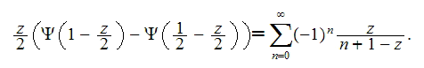 Thus we arrive at an identity, which shows the value of the product of the two factorial
functions witch have arguments with reversed sign
Thus we arrive at an identity, which shows the value of the product of the two factorial
functions witch have arguments with reversed sign
Here we can interpret the infinite sum on the right hand side as a special case
of the Lerch transcendent Phi
 times z and thus the last identity
can be written as
times z and thus the last identity
can be written as
 Since
Since
 where zeta*(n) is the alternating Riemann
zeta function (also called Dirichlet eta function). Note that zeta*(1) = ln 2 (this
is the classical result for the alternating harmonic series). Thus we arrive at
the identity
where zeta*(n) is the alternating Riemann
zeta function (also called Dirichlet eta function). Note that zeta*(1) = ln 2 (this
is the classical result for the alternating harmonic series). Thus we arrive at
the identity 
A representation as a hypergeometric sum.
Recall the definitions of the generalized factorial powers (Concrete Mathematics,
[5.88]).  In terms
of factorial powers the L-factorial can be represented as
In terms
of factorial powers the L-factorial can be represented as
 |
Note that
and that the summation starts at 1. Using the standard notation for hypergeometric functions we can rewrite this as
 |
An asymptotic expansion of L(x) for x -> -infinity.
An asymptotic expansion of L(x) for x -> -infinity is easily found from the identity L(-z) = g(z) / z!. The function g(x) has the simple expansion
| g(x) = 1 / (4 x) (1 - 1 / (2 x^2) + 1 / x^4 - 17 / (4 x^6)) + O(x^(-8)). |
If we combine this expansion with Stirling's asymptotic expansion of Gamma(x) for x -> + infinity (here formula 6.1.37 from the Handbook of Mathematical Functions)
 , , |
where K = (2 * Pi / e) ^ (1/2) and set the constant C = (Pi * e^3 * 2^5) ^ (-1/2) = 0.22540.., than we arrive at the following asymptotic expansion of L(x) for x -> - infinity (which is useful as soon as x < -2).
 |
Finale: A remark from Karl Weierstraß
Indeed the fact, that the Gamma function becomes infinite at n = 0, -1, -2,... raised discomfort early in the development of the function. In the year 1856 Karl Weierstraß [4] introduced his definition of the Gamma function
Fc(u) = u Product( n = 1 .. infinity, (n / (n+1))^u (1 + u / n) ).
Weierstraß commented:
"Ich möchte für dasselbe die Benennung Factorielle von u und die Bezeichnung Fc(u) vorschlagen, indem die Anwendung dieser Function [...] dem Gebrauch der Gamma-Function deshalb vorzuziehen sein dürfte, weil sie für keinen Werth von u eine Unterbrechung der Stetigkeit erleidet und überhaupt [...] im Wesentlichen den Character einer rationalen ganzen Function besitzt." (See [5].)
However, I think Weierstraß jumped too short in his attempt to cure the shortcomings of Euler's definition. Just to replace Gamma(z) by 1/Gamma(z) is a camouflage [6]. It does not remove the 'Unterbrechung der Stetigkeit' from the Gamma function. I think the list of postulates which will ultimately define the 'true' factorial function will include:
[5*] F(u) and 1/F(u) have no discontinuities.
Happily the L-factorial meets also this postulate (see figure 17).
Fig. 17: log(L(1+x)) [red] and log(1/L(1+x)) [green]
"It is true that a mathematician who is not also something of a poet
will never be a perfect mathematician." (Karl Weierstraß)
S u m m a r y
There are two classes of functions which interpolate the factorial numbers n! = 1,2,6,24,... Those which are continuous and those which are not. In the class of not-continuous functions one stands out: The Euler factorial. What makes this function unique is captured by the Bohr-Mollerup-Artin theorem: to be logarithmically convex.
The other class, the class of continuous interpolating functions, never got much publicity. However, Jacques Hadamard stated one exemplar in 1894 which we reconsidered. When reviewed in relation to the geometric properties we found that Hadamard's function is not logarithmic convex for x > 1.
Since this might be regarded as an aesthetic flaw we redesigned the definition and specified a function L(x) which is 'logarithmic single inflected', what means that it is logarithmic convex for x > C for some C and logarithmic concave for x < C.
At a first glance functions from the two interpolating types seem to have very little in common. But this is not true. So we found the following identity
| L(z) L(-z) / g(z) + g(z) / (z! (-z)!) = 1. |
This identity relates the Euler factorial z! and the L-factorial L(z) by some kind of generalized reflection relation via the function g(x) = (x/2) (Psi(x/2 + 1/2) - Psi(x/2)) - 1/2.
What remains an open question is: What property of a continuous interpolant leads to a unique exemplar? What characterization singles a continuous factorial function out like the Bohr-Mollerup-Artin theorem singles out the Euler factorial?
Philip J. Davis closed his exposition [1] with the remark: "... each generation has found something of interest to say about the gamma function. Perhaps the next generation will also."
Postscript
In September 2006 I thought that my story will end here. But this was not the case. A month later the story continued. Here is the second part, which is centered around the super reflection product.
The super reflection product L(z) z! L(-z) (-z)!.
We will use the abbreviations
| g(z) = (z/2) (Psi(z/2 + 1/2) - Psi(z/2)) - 1/2 |
| s(z) = sin(Pi z) / (Pi z) |
| T(z) = 1 / ( g(z) (1 / s(z) - g(z) ) ) |
The value of T at integers n is to be understood as the limit value (which is 0, except at n = 0, where it is 4). We also set
LL(z) = 1/ T(z),
Now we can prove the super reflection formula
LL(z) = L(z) L(-z) z! (-z)!

Fig. 18: The function LL(z).
Looking at T(z) = 1 / LL(z) we find the function which is plotted in figure 18.
Fig. 19: 1 / LL(x) [red] and (4/Pi) sin(PI x) / tanh(x) [green]
When I showed this plot in the Usenet (de.sci.mathematik) Roland Franzius immediately remarked, that this graph looks like the graph of sin(PI x)/tanh(x). And indeed, it does, up to a scaling factor of 4/PI. In figure 19 the green points indicate some of the small differences.
My answer to Roland was: "Yes, however, it is not equal to sin(PI x)/tanh(x)..." and in the same moment I thought: "... but maybe it should be equal!"
So I had to go back and start all over again...
A second start
But this time things were easy to work out. The formulas given above were the markers on the road. Backtracking the observation LL(x) ~ (4/PI) sin(PI x)/tanh(x) I saw that L(x)L(-x) should be well approximated by tanh(x)/(4x). But L(x) = x! P(x) and L(-x) = (-x)!(1-P(x)) and x!(-x!) = PI x / sin(PI x). Thus what I had to do was to solve the equation
P(z) (1 - P(z)) = sin(PI z) tanh(z) / (4 PI z^2)).
Apart from the constant solutions which are of no interest here there are two solutions, P*(z) and 1 - P*(z), where
| P*(z) = 1/2 + (1/(2z)) sqrt(z^2 + (1 - exp(2z)) sin(PI z) / ((exp(2z) + 1) Pi)). |
It is amazing how little P(z) and P*(z) differ numerically.
Fig. 20: The difference P*(z) - P(z).
So we now can replay our game with the definition
| L*(z) = z! P*(z) |
There is no use to plot L*(z) because it looks indistinguishable like the plot of L(z) given above (within the resolution of this media).
The characteristics of L*(z)
First of all, L*(n) = n! if n > 0 is an integer. This is evident. Next it can be easily verified, that the connection with the trigonometric resp. hyperbolic functions do hold, as we aimed at.
| L*(z) L*(-z) = tanh(z) / (4 z) |
| 1 / ( L*(z) L*(-z) z! (-z)! ) = (4 / PI) sin(PI z) / tanh(z) |
Note again, that if we replace L*(z) by L(z) in these identities, we still have good approximations, the error of which rapidly goes to 0 if z goes to +/- infinity.
According to our setup the next important question is: Is L*(x) logarithmic single inflected? So we have to look at V*(x) = (log(L*(x)))''. The answer is 'yes', as a little exercise shows.
A P P E N D I X
Appendix I: The Bohr-Mollerup-Artin Theorem
We give a precise formulation of the Bohr-Mollerup-Artin theorem.
Def.: A real valued function f on (a, b) is convex if
f(cx + (1-c)y) <= cf(x) + (1-c)f(y)
for x, y in (a, b) and 0 < c < 1. A positive function f on (a, b) is logarithmically convex if log f is convex on (a, b).
Theorem. If f is a function on x > 0 and
(0) f(x) > 0 for all x,
(1) f(1) = 1,
(2) f(x + 1) = x f(x) for all x and
(3) f is logarithmically convex,
then f(x) = Gamma(x) for x > 0.
Appendix II: Some special values...


 ...and
more special values (n>0 integer):
...and
more special values (n>0 integer):
L(-n) = g(n) / n! = (-1)^n ( r(n) / n! - ln(2) / (n-1)! )


Appendix III: Series expansions (at x=0) for the factorial functions


| c0 | +0.5 | a0 | +1.0 | b0 | +0.25 |
| c1 | +0.4045393481 | a1 | -0.5772156649 | b1 | 0. |
| c2 | +0.0944325870 | a2 | -0.6558780715 | b2 | -0.0692194972 |
| c3 | -0.0068168967 | a3 | +0.0420026350 | b3 | 0. |
| c4 | -0.0004065045 | a4 | +0.1665386114 | b4 | +0.0140264149 |
| c5 | +0.0052559323 | a5 | +0.0421977346 | b5 | 0. |
| c6 | +0.0025682064 | a6 | -0.0096219715 | b6 | -0.0018075010 |
| c7 | +0.0004731225 | a7 | -0.0072189432 | b7 | 0. |
| c8 | -0.0000169945 | a8 | -0.0011651676 | b8 | +0.0001570804 |
| c9 | -0.0000256306 | a9 | +0.0002152417 | b9 | 0. |
| c10 | -0.0000040188 | a10 | +0.0001280503 | b10 | -0.0000097537 |
| c11 | +0.0000004787 | a11 | +0.0000201348 | b11 | 0. |
| c12 | +0.0000003126 | a12 | -0.0000012505 | b12 | +0.0000004530 |
| c13 | +0.0000000565 | a13 | -0.0000011330 | b13 | 0. |
| c14 | +0.0000000023 | a14 | -0.0000002056 | b14 | -0.0000000163 |
| c15 | -0.0000000011 | a15 | -0.0000000061 | b15 | 0. |
A bound for the absolute error of this approximation of L(x) for
 is given by
 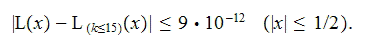 The same bound applies for the given approximation to
 in this range.
Appendix IV: Exercises
Prove the identity a=b, which is made up of two representations of L(z)(-z)!.

Appendix IV:
A C# implementation of the L-factorial.
1: using System;
2:
3: namespace AlternateFactorials {
4:
5: class LuschnyFactorial {
6:
7: public static double Psi(double x)
8: {
9: if (x <= 0 && x == Math.Round(x))
10: return double.NaN;
11:
12: if (x < 0) // reflection formula
13: {
14: double psi = Psi(1.0 - x);
15: double piCotpix = -Math.PI/Math.Tan(-Math.PI*x);
16: return psi - piCotpix;
17: }
18:
19: if (x <= 1e-6)
20: {
21: const double D1 = -0.57721566490153286;
22: const double D2 = 1.6449340668482264365;
23: return D1 + D2 * x - 1.0 / x;
24: }
25:
26: double result = 0.0;
27: const double C = 12.0;
28: while (x < C)
29: {
30: result = result - 1.0 / x;
31: x = x + 1.0;
32: }
33:
34: double r = 1.0 / x;
35: result = result + Math.Log(x) - 0.5 * r;
36: r = r * r;
37:
38: const double S3 = 1.0 / 12.0;
39: const double S4 = 1.0 / 120.0;
40: const double S5 = 1.0 / 252.0;
41: const double S6 = 1.0 / 240.0;
42: const double S7 = 1.0 / 132.0;
43: r *= S3-(r*(S4-(r*(S5-(r*(S6-(r*S7)))))));
44:
45: return result - r;
46: }
47:
48: public static double LnFactorial(double z)
49: {
50: //const double a0 = 1.0 / 12.0;
51: //const double a1 = 1.0 / 30.0;
52: //const double a2 = 53.0 / 210.0;
53: //const double a3 = 195.0 / 371.0;
54: //const double a4 = 22999.0 / 22737.0;
55: //const double a5 = 29944523.0 / 19733142.0;
56: //const double a6 = 109535241009.0 / 48264275462.0;
57: const double a0 = 0.0833333333333333333333333;
58: const double a1 = 0.0333333333333333333333333;
59: const double a2 = 0.252380952380952380952381;
60: const double a3 = 0.525606469002695417789757;
61: const double a4 = 1.01152306812684171174737;
62: const double a5 = 1.51747364915328739842849;
63: const double a6 = 2.26948897420495996090915;
64:
65: const double sqrt2Pi = 0.91893853320467274;
66:
67: double Z = z + 1;
68: return sqrt2Pi + (Z - 0.5) * Math.Log(Z) - Z +
69: a0/(Z+a1/(Z+a2/(Z+a3/(Z+a4/(Z+a5/(Z+a6/Z))))));
70: }
71:
72: public static double Factorial(double x)
73: {
74: if (x < 0 && x == Math.Round(x))
75: return double.NaN;
76: if (0 == x) return 1.0;
77:
78: double y = x;
79: double p = 1;
80: while (y < 8) { p = p * y; y = y + 1.0; }
81: double r = Math.Exp(LnFactorial(y));
82: if (x < 8) { r = (r * x) / (p * y); }
83: return r;
84: }
85:
86: public static double LFactorial(double x)
87: {
88: if (x == 0) return 0.5;
89:
90: double y = x < 0 ? -x * 0.5 : x * 0.5;
91: double G = y * (Psi(y + 0.5) - Psi(y)) - 0.5;
92:
93: if (x < 0)
94: {
95: return G / Factorial(-x);
96: }
97:
98: y = Math.PI * x;
99: double S = Math.Sin(y) / y;
100:
101: return (1 - S * G) * Factorial(x);
102: }
103:
104: }}
Some Maple snippets.
R E F E R E N C E S
[0] See my page "The early history of the factorial function (gamma function)".
[1] There is an excellent exposition which everyone interested in the Gamma function must read: Philip J. Davis: "Leonhard Euler's Integral: A Historical Profile Of The Gamma Function." Am. Math. Monthly 66, 849-869 (1959). However, also note a very serious error of Davis which is discussed here.
[2] Because the paper of Hadamard is not easily accessible I wrote it up in TeX. Here you can download Hadamard's paper "Sur L'Expression Du Produit 1.2.3...(n-1)... Par Une Fonction Entière". Note: I silently corrected a typographical error in formula (2).
[3] Žarko Mijajlović, Branko Malešević: "Differentially Transcendental Functions", arXiv:math.GM/0412354 v3, 9 Feb 2006. Note the error in the definition of Hadamard's function on page 8, Gamma(z-1) instead of Gamma(1-z).
[4] Karl Weierstraß, "Über die Theorie der analytischen Facultäten", Journ. reine angew. Math. 51, 1-60 (1856), Math. Werke 1, 153-221
[5] Translation: "I would like to suggest the term 'factorial of u' and the notation Fc(u) for the same, as the application of this function might have to be preferred to the use of the gamma function [...], because it does not suffer from an interruption of the continuity at any value of u and actually [...] possesses essentially the characteristics of a rational entire function."
[6] Weierstraß' suggestion survived down to the present day in the definition of the Gamma function, as given by many authors. For example Graham, Knuth and Patashnik introduce the Gamma function in Concrete Mathematics as follows: "Here's one of the most useful definitions of z!, actually a definition of 1/z!. 1/z! = lim(n->infinity, binomial(n + z, n)n^(-z))".
[7] The definition of the L-factorial function L(x) was given on this webpage in September 2006. The definition of the L*-factorial function L*(x) was given on this webpage in October 2006. I am not aware that these definitions appeared somewhere else prior to this date. Please let me know if I am mistaken.
Added in 2010.
- In 2009 Horst Alzer proved that Hadamard’s gamma function is superadditive:
H(x) + H(y) ≤ H(x + y) for all real numbers x, y with x, y ≥ 1.5031. A superadditive property of Hadamard’s gamma function. - Some discussions on the web overlooked that the Bohr-Mollerup-Artin theorem only characterizes the real gamma function for x > 0. Hadamard was interested in the complex gamma function as the title of his paper clearly indicates. A beautiful characterization of the complex gamma function does exist, it is Wielandt's theorem, found only many years after the Bohr-Mollerup-Artin theorem. See Reinhold Remmert, Wielandt's Theorem About the Γ-Function, Am. Math. Monthly, Vol. 103 (1996), 214-220.
- Postscript: The purpose of this article was to ask if there are other "interesting" extensions of the factorial function, not to put forward the absurd proposal to replace the Bernoulli-Euler gamma function. I saw some discussions on the web which seem to completely misunderstand its intention; perhaps the somewhat provocative title of this page and a very superficial reading is the cause.
Acknowledgment: I would like to thank David W. Cantrell to draw my attention to Hadamard's definition.


 Back to the Homepage of Factorial Algorithms.