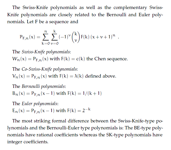
The Swiss-Knife polynomials

Representations of classical numbers

More on this can be found here: Decompositions of the Euler, Bernoulli, Genocchi, Springer and tangent numbers.

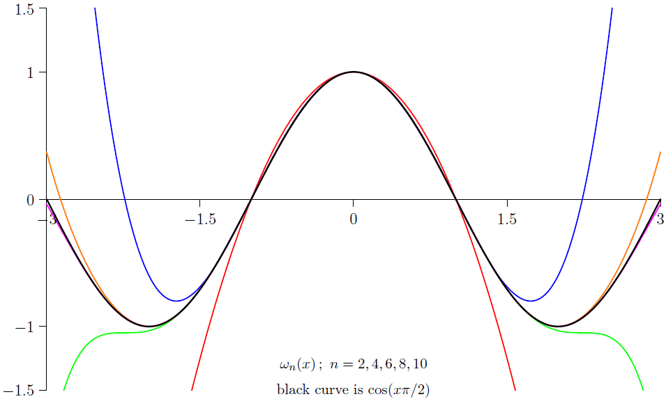
The sinusoidal character of the polynomials

The scaled Swiss-Knife polynomials are defined as

$\omega_n(x) = W_n(x)\,/\,|\,W_n([n\ \operatorname{odd}])\,|$

Plotting ω_n(x) shows the sinusoidal behavior of these polynomials, which is easily overlooked in the non-scaled form. For odd index ω_n(x) approximates sin(xΠ/2) and for even index cos(xΠ/2) in an interval enclosing the origin. This observation expands the observation that the Euler and Bernoulli number have Π as a common root ( cf. e.g.) to an continuous scale.

But much more is true: the domain of sinusoidal behavior gets larger and larger as the degree of the polynomials grows. In fact ω_n(x) shows, in an asymptotical precise sense, sinusoidal behavior in the interval [-2n/Πe, 2n/Πe].

From these observations follows the regular behavior of the real roots of the Swiss-Knife polynomials. For example the roots of ω_n(x) are close to the integer lattices: {±0,±2,±4,...} if n is odd and {±1,±3,±5,...} if n is even.

Plots of the scaled Swiss-Knife polynomials

Maple Code

The Swiss-Knife polynomials by definition.

SwissKnifePolynomial := proc(n, x) local v, k, pow, chen; 
pow := (a,b) -> if a = 0 and b = 0 then 1 else a^b fi;
chen := m -> if irem(m+1,4) = 0 then 0 
else 1/((-1)^iquo(m+1,4)*2^iquo(m,2)) fi;  
add(add((-1)^v*binomial(k,v)*pow(v+x+1,n)*chen(k),v=0..k),k=0..n)
end:

Swiss-Knife polynomials, triangle of coefficients:

for i from 0 to 9 do
p := sort(expand(SwissKnifePolynomial(i,x)));
print(seq(coeff(p,x,i-j),j=0..i)): od:

                    1
                   1, 0
                 1, 0, -1
               1, 0, -3, 0
              1, 0, -6, 0, 5
           1, 0, -10, 0, 25, 0
         1, 0, -15, 0, 75, 0, -61
      1, 0, -21, 0, 175, 0, -427, 0
   1, 0, -28, 0, 350, 0, -1708, 0, 1385
 1, 0, -36, 0, 630, 0, -5124, 0, 12465, 0

A representation of the Swiss-Knife polynomials by a single sum.

SKPolynomial := proc(n,x) local k;
add(binomial(n,k)*euler(k)*x^(n-k),k=0..n) end;

for n from 0 to 7 do SKPolynomial(n,x) od;

              1
              x
           x^2 - 1
         x^3 - 3 x
       x^4 - 6 x^2 + 5
     x^5 - 10 x^3 + 25 x
   x^6 - 15 x^4 + 75 x^2 - 61
 x^7 - 21 x^5 + 175 x^3 - 427 x

An exponential generating function for the SKPolynomials.

G := (x, t) -> 2*exp(x*t)/(exp(t)+exp(-t));

Sum of alternating powers

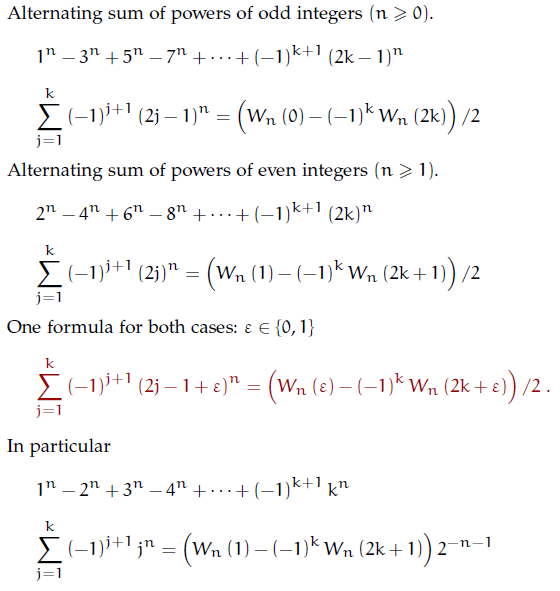
Note that all this can be done with integer arithmetic only. So why use some kind of generalized Bernoulli polynomials which are more complicated and use rational arithmetic? Even an evaluation with Euler polynomials has to use rational arithmetic because the coefficients of the Euler polynomials are rational numbers -- in contrast to the coefficients of the Swiss-Knife polynomials which are integers. And... it's just nice to know that it can be done by conceptual simpler polynomials.

It seems much more interesting to ask how much of the functionality the generalized Bernoulli or Euler polynomials provide can be reconstructed in terms of the Swiss-Knife polynomials.

A surprising connection with the von Mangoldt function

The greatest common divisor of the nonzero coefficients of the decapitated Swiss-Knife polynomials is exp(Lambda(n)), where Lambda(n) is the von Mangoldt function for odd primes [OEIS-A155457].

seq(igcd(coeffs(expand(SwissKnifePolynomial(i,x)-x^i))),i=2..49);

1, 3, 1, 5, 1, 7, 1, 3, 1, 11, 1, 13, 1, 1, 1, 17, 1, 19, 1, 1, 1, 23, 1, 5, 1, 3, 1, 29, 1, 31, 1, 1, 1, 1, 1, 37, 1, 1, 1, 41, 1, 43, 1, 1, 1, 47, 1, 7

The complementary Swiss-Knife Polynomials

Added 2009/07/09

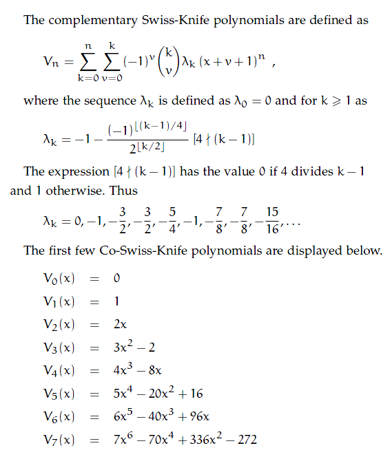
The Swiss-Knife polynomials are complementary to the polynomials defined here. Adding both gives polynomials which we will study below.

Maple Code

The Co-Swiss-Knife polynomials by definition.

CoSwissKnifePolynomial := proc(n,x) 
local v, k, pow, iver, lambda; 
iver := k -> if k mod 4 <> 0 then 1 else 0 fi:
lambda := k -> `if`(k=0,0,-1-iver(k-1)*(-1)^iquo(k-1,4)/2^iquo(k,2));
pow := (a, b) -> if a = 0 and b = 0 then 1 else a^b fi;
add(add((-1)^v*binomial(k,v)*pow(x+v+1,n)*lambda(k),v=0..k),
k=0..n) end:

Co-Swiss-Knife polynomials, triangle of coefficients:

for i from 0 to 9 do
p := sort(expand(CoSwissKnifePolynomial(i,x)));
print(seq(coeff(p,x,i-j),j=0..i)): od:

                    0
                   0, 1
                 0, 2, 0
               0, 3, 0, -2
              0, 4, 0, -8, 0
           0, 5, 0, -20, 0, 16
          0, 6, 0, -40, 0, 96, 0
      0, 7, 0, -70, 0, 336, 0, -272
    0, 8, 0, -112, 0, 896, 0, -2176, 0
0, 9, 0, -168, 0, 2016, 0, -9792, 0, 7936

A representation of the Co-Swiss-Knife polynomials by a single sum.

CoSKPolynomial := proc(n,x) local k,pow;
pow := (n,k) -> `if`(n=0 and k=0,1,n^k);
add(binomial(n,k)*euler(k)*pow(x+1,n-k),k=0..n)-pow(x,n) end:

for n from 0 to 7 do CoSKPolynomial(n,x) od;

           0
           1
          2*x
        3*x^2-2
       4*x^3-8*x
    5*x^4-20*x^2+16
   6*x^5-40*x^3+96*x
7*x^6-70*x^4+336*x^2-272

An exponential generating function for the CoSKPolynomials.

G := (x, t) -> exp(x*t)*(exp(2*t)-1)/(exp(2*t)+1);

A comparison with the Bernoulli and Euler polynomials.

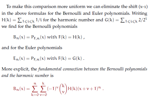
Bernoulli polynomials and harmonic number.

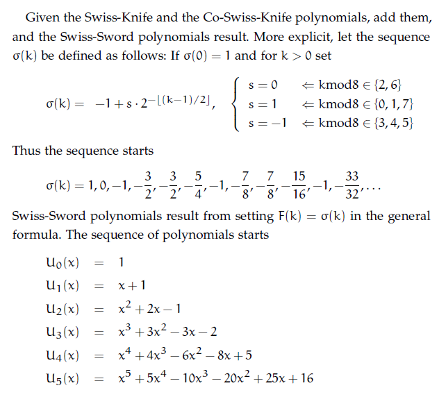
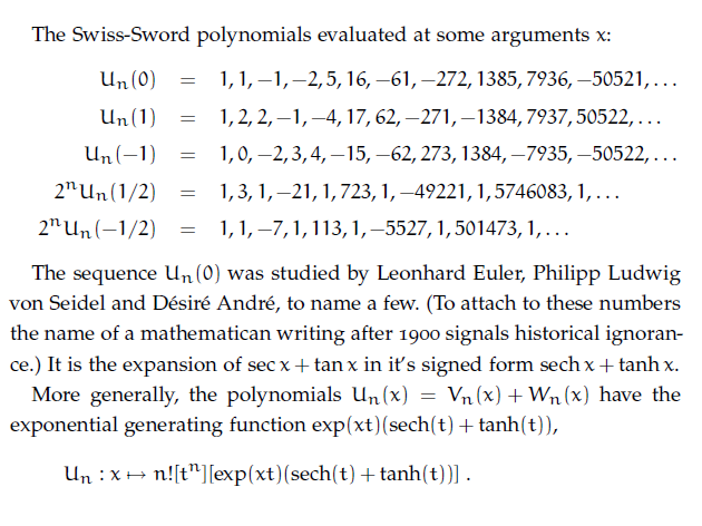
The Swiss-Sword polynomials.

A sword has a blade with two cutting edges. So if we combine the cutting edge of a Swiss-Knife with the cutting edge of a Co-Swiss-Knife we have a Zweihänder in our scabbard and earn twice the pay of a common combinatorialist as a Doppelsöldner of Math.

References

Euler, Leonhard (1735), "De summis serierum reciprocarum", Opera Omnia I.14, E 41, 73-86; On the sums of series of reciprocals, arXiv:math/0506415v2 (math.HO).
J. Worpitzky, "Studien über die Bernoullischen und Eulerschen Zahlen.", Journal für die reine und angewandte Mathematik, 94 (1883), 203--232.
Kwang-Wu Chen, "Algorithms for Bernoulli numbers and Euler numbers.", Journal of Integer Sequences, 4 (2001), [01.1.6].

Rational Trees	Factorial Functions	Eulerian Polynomials	vonStaudt Primes	Irregular Primes	Generalized Binomial
Bernoulli Manifesto	Partitions Stirling	Zeta Polynomials	Perfect Rulers	Swinging Primes	Clausen Numbers
Hadamard Gamma	History Factorial	Permutation Trees	Swiss Knife	Swinging Factorial	Worpitzky Triangle

Author: Peter Luschny (2008-12-30). License: Creative Commons Attribution-ShareAlike 3.0 Unported License.

Swiss-Knife	A153641
Co-Swiss-Knife	A162660
Swiss-Sword	A109449